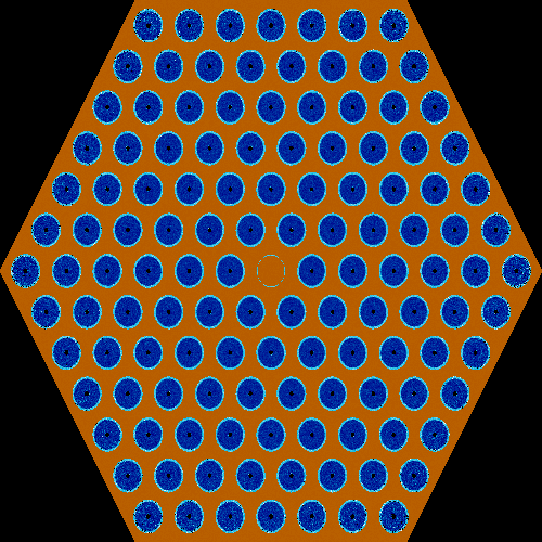
Regular Hex Mesh coolant IFC example
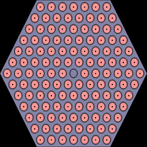
Input example for single assembly regular mesh based interface for coolant using hexagonal mesh. On-the-fly interpolation of thermal scattering data is used for the hydrogen-1 in coolant (see therm).
Remember to add cross section libraries to the main input using set acelib.
Contents
Files
Main input
set title "Regular hex mesh interface input"

%%%%%%%%%%%%%%%%%%%%%%%%%%%%
% --- Material definitions %
%%%%%%%%%%%%%%%%%%%%%%%%%%%%

mat fuel -10.31341 rgb 255 150 150
U-234.03c 5.0131e-06
U-235.03c 5.7503e-04
U-238.03c 2.2625e-02
O-16.03c 4.5895e-02
O-17.03c 1.7482e-05

mat zirc  -6.55 rgb 100 100 100
O-16.03c 3.0743e-04
O-17.03c 1.1711e-07
%O-18.03c 6.3176e-07
Cr-50.03c 3.2962e-06
Cr-52.03c 6.3564e-05
Cr-53.03c 7.2076e-06
Cr-54.03c 1.7941e-06
Fe-54.03c 8.6699e-06
Fe-56.03c 1.3610e-04
Fe-57.03c 3.1431e-06
Fe-58.03c 4.1829e-07
Zr-90.03c 2.1827e-02
Zr-91.03c 4.7600e-03
Zr-92.03c 7.2758e-03
Zr-94.03c 7.3734e-03
Zr-96.03c 1.1879e-03
Sn-112.03c 4.6735e-06
Sn-114.03c 3.1799e-06
Sn-115.03c 1.6381e-06
Sn-116.03c 7.0055e-05
Sn-117.03c 3.7003e-05
Sn-118.03c 1.1669e-04
Sn-119.03c 4.1387e-05
Sn-120.03c 1.5697e-04
Sn-122.03c 2.2308e-05
Sn-124.03c 2.7897e-05

mat cool  sum rgb 200 200 255 moder HinWater 1001
H-1.03c 4.9457e-02
H-2.03c 7.4196e-06
O-16.03c 2.4672e-02
O-17.03c 9.3982e-06
%O-18.03c 5.0701e-05

% --- Use on-the-fly interpolation for thermal scattering data
%     lwj3.07t = 474 K / JEFF3.1.1
%     lwj3.09t = 524 K / JEFF3.1.1
%     lwj3.11t = 574 K / JEFF3.1.1

therm HinWater 0 lwj3.07t lwj3.09t lwj3.11t

%%%%%%%%%%%%%%%%%%%%%%%%%%%
% --- Geometry definition %
%%%%%%%%%%%%%%%%%%%%%%%%%%%

surf s01  hexyc 0 0 7
surf s02  pz -50
surf s03  pz  50
surf sINF inf

% --- Core

cell c01 0 fill lPIN -s01 s02 -s03
cell c02 0 outside    s01 s02 -s03
cell c03 0 outside       -s02
cell c04 0 outside             s03

% --- Fuel assembly pin lattice

lat lPIN 2 0.0 0.0 15 15 1.22
ww ww ww ww ww ww ww ww ww ww ww ww ww ww ww
 ww ww ww ww ww ww ww PF PF PF PF PF PF PF ww
  ww ww ww ww ww ww PF PF PF PF PF PF PF PF ww
   ww ww ww ww ww PF PF PF PF PF PF PF PF PF ww
    ww ww ww ww PF PF PF PF PF PF PF PF PF PF ww
     ww ww ww PF PF PF PF PF PF PF PF PF PF PF ww
      ww ww PF PF PF PF PF PF PF PF PF PF PF PF ww
       ww PF PF PF PF PF PF IT PF PF PF PF PF PF ww
        ww PF PF PF PF PF PF PF PF PF PF PF PF ww ww
         ww PF PF PF PF PF PF PF PF PF PF PF ww ww ww
          ww PF PF PF PF PF PF PF PF PF PF ww ww ww ww
           ww PF PF PF PF PF PF PF PF PF ww ww ww ww ww
            ww PF PF PF PF PF PF PF PF ww ww ww ww ww ww
             ww PF PF PF PF PF PF PF ww ww ww ww ww ww ww
              ww ww ww ww ww ww ww ww ww ww ww ww ww ww ww


% --- Pin definitions

%     Empty lattice position

pin ww
cool

%     Fuel pin

pin      PF
void     0.07
fuel     0.3765
void     0.3865
zirc     0.4575
cool

%      Instrumentation tube

pin      IT
cool     0.3850
zirc     0.4400
cool

%%%%%%%%%%%%%%%%%%%%%%%%
% --- Some run options %
%%%%%%%%%%%%%%%%%%%%%%%%

set pop 5000 1000 50

% --- Cross section libraries

%set acelib ""

% --- Geometry plot

plot 3 500 500
plot 1 500 500

% --- Sample temperature and density data in 20 points on z-axis

sample 1 0 0 1 0 0 10 -49.9 49.9

% --- Fission rate / thermal flux plot

mesh    3 500 500
mesh    1 500 500

% --- Interface temperature plot

mesh 10 3 500 500
mesh 10 1 500 500

% --- Include interface for assembly-wise fuel temperature

ifc "./coolant.ifc"
coolant.ifc
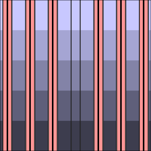
The interface consists of five axial layers from bottom to top. Here the mesh type 5 corresponds to the assembly shape (y-type hexagon, i.e. flat top hexagon) in the input , although a cartesian mesh with large enough bin size in XY-directions could have also been used as there is no variation in the horizontal direction. We let the coolant density decrease from 1 g/cm3 to 0.6 g/cm3 while increasing the coolant temperature from 520 K to 540 K.
2 cool 0
5
0 0 14 -50.0 50.0 1 1 5
-1.0 520
-0.9 525
-0.8 530
-0.7 535
-0.6 540
Output files
input_sample1.m
We used the sample-card to take a sample of the material temperatures and densities on the z-axis to ensure that the interface data is read correctly by Serpent. The contents of this file are
SAMPLE_X = [
 0.00000E+00
];

SAMPLE_Y = [
 0.00000E+00
];

SAMPLE_Z = [
-4.99000E+01 -3.88111E+01 -2.77222E+01 -1.66333E+01 -5.54444E+00  5.54444E+00  1.66333E+01  2.77222E+01  3.88111E+01  4.99000E+01
];

sampled_T = [
 5.20000E+02  5.20000E+02  5.25000E+02  5.25000E+02  5.30000E+02  5.30000E+02  5.35000E+02  5.35000E+02  5.40000E+02  5.40000E+02
];


sampled_T = reshape(sampled_T, [1, 1, 10]);

sampled_rho = [
-1.00000E+00 -1.00000E+00 -9.00000E-01 -9.00000E-01 -8.00000E-01 -8.00000E-01 -7.00000E-01 -7.00000E-01 -6.00000E-01 -6.00000E-01
];


sampled_rho = reshape(sampled_rho, [1, 1, 10]);
Comparing the (Z, T, rho) triplets, we can see that the temperatures and densities are seen by Serpent as we intended. Of course, a much higher resolution could be used in sampling to ensure that the transition between the axial layers happens at the correct position.
Geometry and mesh plots
The geometry plots show the variation in coolant temperature.
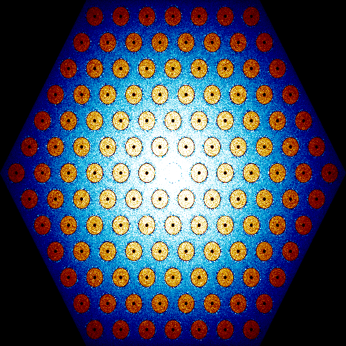
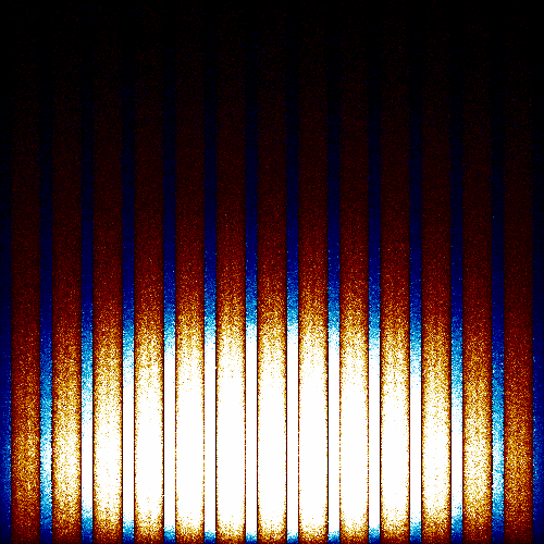
The fission rate mesh plots show the fission rate distribution being mainly in the lower part of the assembly (due to higher moderation).
The temperature mesh plots show (poorly) the variation in the axial coolant temperature. It is easier to check the variation using the sample-card.
