Difference between revisions of "Boundary conditions"
(→Radially infinite, axially finite 3D geometry) |
(→Infinite 2D geometries) |
||
| Line 27: | Line 27: | ||
== Infinite 2D geometries == | == Infinite 2D geometries == | ||
| − | Two types of infinite square lattices created using reflective and periodic boundary conditions are illustrated below, together with a non-repetitive black boundary. The geometry plot is extended beyond the outermost surface, in which case the plot shows the vacuum region as black and applies reflections and translations accordingly. The image captions provide links to particle track animations, which illustrate the behaviour when the boundary is hit. It should be noted that the boundary surface is not plotted, since the material is the same on both sides. | + | In infinite 2D lattice geometries the outside part of the geometry is composed of a single cell filling the space outside the surface at which the boundary conditions are applied. For example: |
| + | |||
| + | <nowiki> | ||
| + | cell 999 0 outside b1</nowiki> | ||
| + | |||
| + | where surface b1 is an infinite square prism. | ||
| + | |||
| + | Two types of infinite square lattices created using reflective and periodic boundary conditions are illustrated below, together with a non-repetitive black boundary. The geometry plot is extended beyond the outermost surface, in which case the plot shows the vacuum region as black and applies reflections and translations accordingly. The image captions provide links to particle track animations, which illustrate the behaviour when the boundary is hit. It should be noted that the boundary surface itself is not plotted, since the material is the same on both sides. | ||
<gallery mode="nolines" widths=320px heights=320px> | <gallery mode="nolines" widths=320px heights=320px> | ||
Revision as of 15:20, 25 February 2016
Boundary conditions are invoked when the particle crosses the boundary from the defined part of the geometry into a region labeled as "outside" in the cell cards. The outcome then depends on the boundary conditions, as defined by the "set bc" option. Serpent provides three types of boundary conditions:
- Black boundary - the particle is killed
- Reflective boundary - the particle is reflected back into the geometry
- Periodic boundary - the particle is moved to the opposite side of the geometry
Reflective and periodic boundary conditions can be used to construct infinite and semi-infinite lattice structures. The way these boundary conditions are handled in Serpent is somewhat different from other Monte Carlo codes. Instead of stopping the neutron at the boundary surface, reflections and translations are handled by coordinate transformations. This limits the outermost boundary to a few specific surface types that form regular lattices. In 2D geometries such surfaces are:
- Square prism ("sqc") - forms a 2D square lattice
- Hexagonal prisms ("hexxc" and "hexxyc") -- form 2D hexagonal lattices
- Rectangular prism ("rect") - forms a 2D rectangular lattice
And in 3D:
- Cube ("cube") - forms a 3D cubical lattice
- Cuboid ("cuboid") - forms a 3D cuboidal lattice
- Truncated hexagonal prisms ("hexxprism" and "hexyprism") - form a 3D hexagonal lattices
Repeated boundary conditions are invoked only on the first surface listed in the "outside" type cells. Since the geometry boundary may consist of additional surfaces, some boundaries may be treated as reflective or periodic, while others are treated as vacuum. In reactor geometries there are typically three possible configurations:
- Infinite 2D geometry
- The geometry has no dependence on the z-coordinate. The outer boundary is defined by one of the 2D surfaces listed above.
- Radially infinite, axially finite 3D geometry
- The outer boundary is defined by one of the 2D surfaces listed above and two axial planes ("pz"). The boundary condition takes effect in the radial direction only, while the axial boundaries are vacuum.
- Infinite 3D geometry
- The outer boundary is defined by one of the 2D surfaces listed above. The boundary condition takes effect in all directions.
These configurations are demonstrated below.
Infinite 2D geometries
In infinite 2D lattice geometries the outside part of the geometry is composed of a single cell filling the space outside the surface at which the boundary conditions are applied. For example:
cell 999 0 outside b1
where surface b1 is an infinite square prism.
Two types of infinite square lattices created using reflective and periodic boundary conditions are illustrated below, together with a non-repetitive black boundary. The geometry plot is extended beyond the outermost surface, in which case the plot shows the vacuum region as black and applies reflections and translations accordingly. The image captions provide links to particle track animations, which illustrate the behaviour when the boundary is hit. It should be noted that the boundary surface itself is not plotted, since the material is the same on both sides.
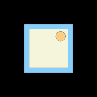
Vacuum boundary conditions ("set bc 1", xy-plot). See animated particle tracks.
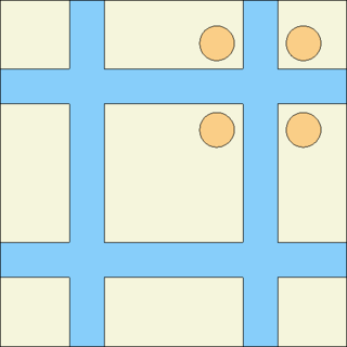
Reflective boundary conditions ("set bc 2", xy-plot). See animated particle tracks.
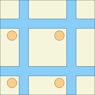
Periodic boundary conditions ("set bc 3", xy-plot). See animated particle tracks.


Serpent allows using reflective and periodic boundary conditions for both square and hexagonal prisms, although it should be noted that a reflective boundary with a non-symmetrical hexagonal cell makes physically no sense.
Radially infinite, axially finite 3D geometry
Three-dimensional model of a fuel assembly in an infinite lattice is an example of a geometry that is radially infinite and axially finite. The outer boundary of such geometry is formed by the surface at which the repeated boundary conditions are applied, and two axial planes that the define the bottom and top of the geometry model. The outside cells could then be defined as:
cell 997 0 outside  b1  b2 -b3
cell 998 0 outside -b2
cell 999 0 outside  b3
where surfaces b1, b2 and b3 are an infinite square prism and planes forming the bottom and the top of the geometry, respectively. It is important that the surface at which the boundary conditions are applied is listed first.
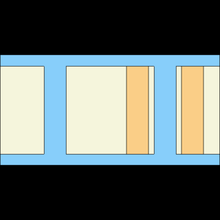
Reflective boundary conditions ("set bc 2", yz-plot). See animated particle tracks.
