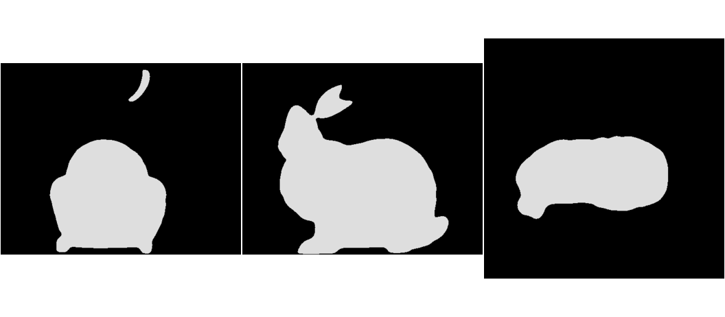
Rotating Translating STL Bunny
This example demonstrates the use of time-dependent transformations in the context of STL-objects. Time dependent transformations are also applicable to other Serpent objects.
Input
The main input file:
%%%%%%%%%%%%%%%%%%%%%%%%%%%%%%%%%%%%%%%%%
% --- Geometry and material information %
%%%%%%%%%%%%%%%%%%%%%%%%%%%%%%%%%%%%%%%%%

% --- Box containing bunny:

surf 1 cyl 0.0 0.0 17.0 -0.1 27

cell 1 0 fill 1  -1 % Fill box with mesh based universe
cell 2 0 outside  1 % Outside of the box is outside

% --- Create the background universe (filled with void)

surf 3 inf
cell 4 2 void -3

% --- Create the STL-bunny

solid 2 1 2                        % type, universe, bacground universe
10 4 5 4 3 2                       % search mesh split, depth and sizes
1 1E-5                             % ray test, merge radius
body fuel fuel fuel                % solid name, cell name, material name
file fuel "bunny.stl" 1.00 0 0 0   % body name, file, scaling factor, origin

% --- Composition for bunny:

mat fuel  4.7984E-02 rgb 222 222 222
92235.03c 4.4994E-02
92238.03c 2.4984E-03
92234.03c 4.9184E-04

%%%%%%%%%%%%%%%%%%%%%%%%%%%%%%%%%%%%%%%%%%%%%%%%%%%%%%%
% --- Add up and down translations using acceleration %
%%%%%%%%%%%%%%%%%%%%%%%%%%%%%%%%%%%%%%%%%%%%%%%%%%%%%%%

% --- Upwards acceleration of 1e13 cm/s^2 from 0.0 s to 0.9e-6 s

transa u 1 tlim 0 0.9e-6      3 0 0  1e13

% --- Downwards acceleration of 1e13 cm/s^2 from 0.9e-6 s to 2.7e-6 s
%     First for slowing down and then for acceleration.

transa u 1 tlim 0.9e-6 2.7e-6 3 0 0 -1e13

% --- Upwards acceleration of 1e13 cm/s^2 from 2.7e-6 s to 3.6e-6 s
%     For slowing down

transa u 1 tlim 2.7e-6 3.6e-6 3 0 0  1e13

%%%%%%%%%%%%%%%%%%%%%%%%%%%%%%%%%%%%%%%%
% --- Add rotations using acceleration %
%%%%%%%%%%%%%%%%%%%%%%%%%%%%%%%%%%%%%%%%

% --- Angular acceleration to the negative mathematical direction
%     around axis defined by vector starting from 0.0 0.0 0.0 with i, j, k
%     components 0.0 0.0 1.0. Magnitude of angular acceleration is
%     1.11111111111111e+14 degrees/s^2 from 0.0 s to 1.8e-6 s
%     (results in rotation of 180 degrees in 1.8 e-6 s)
%     NOTE: The signs are inverted for Serpent 2.1.29 (positive sign corresponds to
%     negative rotation)

transa u 1 tlim 0 1.8e-6      3 rot 0.0 0.0 0.0 0.0 0.0 1.0 1.11111111111111e+14

% --- Angular acceleration to the positive mathematical direction
%     around axis defined by vector starting from 0.0 0.0 0.0 with i, j, k
%     components 0.0 0.0 1.0. Magnitude of angular acceleration is
%     1.11111111111111e+14 degrees/s^2 from 1.8e-6 s to 3.6e-6 s

transa u 1 tlim 1.8e-6 3.6e-6 3 rot 0.0 0.0 0.0 0.0 0.0 1.0 -1.11111111111111e+14

%%%%%%%%%%%%%%%%%%%%%%%%%%%%%%
% --- Run & plot parameters: %
%%%%%%%%%%%%%%%%%%%%%%%%%%%%%%

% --- Link cross section libraries

set acelib "/home/vvvillehe/XSdata/xsdir0K"

% --- Link dynamic source (this way the geometry will be plotted for each time interval)

set dynsrc "./source" 1

% --- Define time-interval structure to be used with the simulation
%     180 equally wide time-intervals between 0 s and 3.6e-6 s

tme simutime 2 180 0.0 3.6e-6

% --- Simulate a small number of neutrons just to get the plots

set nps 5000 10 simutime

% --- Increase the precursor and neutron buffer sizes for the dynamic simulation

set pbuf 40
set nbuf 40

% --- Create plots for each plot plane

plot 1 500 399
plot 2 500 399
plot 3 500 500
Additional input-files:
- bunny.stl
- The dynamic source files (source.*) need to be created using a separate criticality source simulation.
Running
NOTE: Since the delayed neutron precursors are not rotated and/or translated alongside with the geometry, some of them will fall outside of the bunny during some parts of the simulation and be emitted from the void-part of the geometry instead. This will lead to a number of warning messages such as
***** Tue Jun 20 14:58:13 2017 (seed = 1497959831)
Warning message from function SamplePointDelnu:

Precursor is not in material?

 x = -2.443193E+00, y = -4.201429E+00, z = 9.463751E+00
 Cell name 4
Output
The following animation can be compiled from the 180 plots rendered for each of the three plotting planes:

Notes
- The transformations are updated at time-interval boundaries, which means that the geometry is static for each time-interval.
- The positions of neutrons and precursors are not updated as the transformations are updated.
- In external source simulations (no delayed neutrons, no coupled calculation) the geometry plots are only produced for the first time interval, although the transformations are applied similarly.