Coupled transient tutorial with MSCS
This tutorial describes how to use Serpent 2.1.29 to solve a simple reactivity insertion transient for a 3x3 rod unit cell with a central AIC control rod. We will solve the coupled neutronics-fuel temperature problem for an accidental fast removal and return of the control rod. We will not solve heat conduction in the fuel, but will use an adiabatic approximation instead: all heat is modelled as remaining at the place of deposition.
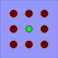
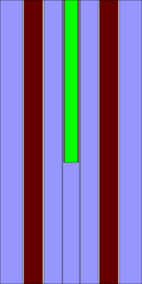
The XY and XZ cuts of the geometry we want to simulate are shown below:
The details of the transient we want to simulate follow: In the beginning of the transient, the system (made critical by soluble boron) is operating at a power level of 1.0 W with the delayed neutron precursors at their stable concentrations. The control rod is removed from the system with an instantaneous upward velocity of 100 000 cm/s, which is maintained until the control rod is completely removed from the geometry. After this, the control rod is inserted back with 5% of the removal speed until the initial position is reached again.
Initial input
In order to simulate the transient, we will need to first generate the source distributions for neutrons and delayed neutron precursors in the beginning of the transient. As we want to start the transient from the critical state (starting from subcritcal or supercritical states is not currently supported), we will need to create a critical model of our system.
Let's start with the following input (you'll have to link to your own acefile):
Initial input for 3x3 rod 3D unit cell
/****************
 * Main options *
 ****************/

% --- Link XS-libraries

set acefile "REPLACE_ACEFILE_NAME_HERE"

% --- Neutron population and criticality cycles:

set pop 10000 50 50

% --- Total power for normalization (1 W):

set power 1

% --- Use reflective boundary condition in XY, black in Z

set bc 2 2 1

% --- Add geometry plots

plot 2 500 1000
plot 3 500 500

% --- Add mesh plots (flux + fission power)

mesh 3 500 500
mesh 2 500 1000

% --- Temperature mesh plots

mesh 10 3 500 500
mesh 10 2 500 1000

/*******************
 * Pin definitions *
 *******************/

% --- Empty lattice position:

pin 99
cool

% --- Fuel pins (same type but treated separately)

pin 1
fuel1  0.60579
void   0.62103
Zirc2  0.71501
cool

pin 2
fuel1  0.60579
void   0.62103
Zirc2  0.71501
cool

% --- Control rod

pin CR
AgInCd  0.43310
void    0.43688
ssteel  0.48387
cool    0.56134
zirc    0.60198
cool

% --- Control rod guide thimble

pin GT
cool    0.56134
zirc    0.60198
cool

% --- Control rod bottom surface

surf sCR pz 0.0

% --- Move control rod surface to starting position

trans s sCR 0 0 -3.54

% --- Control rod universe C definition

cell CRb C fill GT -sCR
cell CRt C fill CR  sCR

/***********************
 * Geometry definition *
 ***********************/

% --- Assembly lattice

lat 100 1  0.0  0.0 5 5 2.5
99 99 99 99 99
99  1  2  1 99
99  2  C  2 99
99  1  2  1 99
99 99 99 99 99

% --- Geometry boundary (50 cm high cuboid)

surf  9  cuboid  -4.6875 4.6875 -4.6875 4.6875 -25 25

% --- Cell definitions:

cell  1  0 fill 100  -9          % Pin lattice
cell 99  0 outside    9          % Outside world

/************************
 * Material definitions *
 ************************/

% --- Fuel materials:

% Fuel1 3.6 wt % enrichment (double density)
mat fuel1   -10.307 tmp 300 rgb 100 0 0
92235.03c	-0.03173362
92238.03c	-0.84975585
8016.03c        -0.11851053

% --- "Zircaloy-2" [PNNL-15870, Rev. 1]
% Xe18 commented because of lack of XS data

mat Zirc2 -6.56 tmp 300 rgb 200 200 200
 8016.03c  -1.19376E-03
 8017.03c  -4.83282E-07
24050.03c  -4.16117E-05
24052.03c  -8.34483E-04
24053.03c  -9.64457E-05
24054.03c  -2.44600E-05
26054.03c  -5.62862E-05
26056.03c  -9.16258E-04
26057.03c  -2.15389E-05
26058.03c  -2.91667E-06
28058.03c  -3.35317E-04
28060.03c  -1.33612E-04
28061.03c  -5.90496E-06
28062.03c  -1.91358E-05
28064.03c  -5.03067E-06
40090.03c  -4.98111E-01
40091.03c  -1.09835E-01
40092.03c  -1.69731E-01
40094.03c  -1.75753E-01
40096.03c  -2.89183E-02
50112.03c  -1.27668E-04
50114.03c  -8.84175E-05
50115.03c  -4.59485E-05
50116.03c  -1.98205E-03
50117.03c  -1.05596E-03
50118.03c  -3.35857E-03
50119.03c  -1.20129E-03
50120.03c  -4.59450E-03
50122.03c  -6.63830E-04
50124.03c  -8.43778E-04

% --- Zircaloy for control rod
mat zirc   -6.56000E+00 tmp 300 rgb 200 200 200
 8016.03c  -1.19376E-03
 8017.03c  -4.83282E-07
24050.03c  -4.16117E-05
24052.03c  -8.34483E-04
24053.03c  -9.64457E-05
24054.03c  -2.44600E-05
26054.03c  -5.62862E-05
26056.03c  -9.16258E-04
26057.03c  -2.15389E-05
26058.03c  -2.91667E-06
28058.03c  -3.35317E-04
28060.03c  -1.33612E-04
28061.03c  -5.90496E-06
28062.03c  -1.91358E-05
28064.03c  -5.03067E-06
40090.03c  -4.98111E-01
40091.03c  -1.09835E-01
40092.03c  -1.69731E-01
40094.03c  -1.75753E-01
40096.03c  -2.89183E-02
50112.03c  -1.27668E-04
50114.03c  -8.84175E-05
50115.03c  -4.59485E-05
50116.03c  -1.98205E-03
50117.03c  -1.05596E-03
50118.03c  -3.35857E-03
50119.03c  -1.20129E-03
50120.03c  -4.59450E-03
50122.03c  -6.63830E-04
50124.03c  -8.43778E-04

% --- "Steel, Stainless 304" [PNNL-15870, Rev. 1]

mat ssteel -8.00000E+00 tmp 300 rgb 100 100 100
 6012.03c  -3.95366E-04
% 6013.03c  -4.63372E-06
14028.03c  -4.59332E-03
14029.03c  -2.41681E-04
14030.03c  -1.64994E-04
15031.03c  -2.30000E-04
16032.03c  -1.42073E-04
16033.03c  -1.15681E-06
16034.03c  -6.75336E-06
16036.03c  -1.68255E-08
24050.03c  -7.93000E-03
24052.03c  -1.59029E-01
24053.03c  -1.83798E-02
24054.03c  -4.66139E-03
25055.03c  -1.00000E-02
26054.03c  -3.96166E-02
26056.03c  -6.44901E-01
26057.03c  -1.51600E-02
26058.03c  -2.05287E-03
28058.03c  -6.21579E-02
28060.03c  -2.47678E-02
28061.03c  -1.09461E-03
28062.03c  -3.54721E-03
28064.03c  -9.32539E-04

% --- AIC from BEAVRS

mat AgInCd -10.160000 tmp 300 rgb 5 255 5
Ag-107.03c 2.3523e-02
Ag-109.03c 2.1854e-02
In-113.03c 3.4291e-04
In-115.03c 7.6504e-03
Cd-106.03c 3.4019e-05
Cd-108.03c 2.4221e-05
Cd-110.03c 3.3991e-04
Cd-111.03c 3.4835e-04
Cd-112.03c 6.5669e-04
Cd-113.03c 3.3257e-04
Cd-114.03c 7.8188e-04
Cd-116.03c 2.0384e-04

% --- Coolant (0% void fraction):

mat cool     -0.99999  moder lwtr 1001 tmp 300 rgb 150 150 255
 1001.03c     0.66667
 8016.03c     0.33333

% --- Thermal scattering data for light water:

%(HinH20 at 273K)
therm lwtr lwj3.00t
Running the simulation will produce the geometry plots already shown above and also tell us something about the estimated k-eff of the system:
------------------------------------------------------------

Serpent 2.1.29 -- Static criticality source simulation

Input file: "input"

Active cycle   50 / 50  Source neutrons :  9743

Running time :                  0:02:08
Estimated running time :        0:02:08
Estimated running time left :   0:00:00

Estimated relative CPU usage :   296.0%

k-eff (analog)    = 0.99947 +/- 0.00173  [0.99609  1.00285]
k-eff (implicit)  = 0.99942 +/- 0.00090  [0.99765  1.00120]

(O4) (OMP=3)
------------------------------------------------------------
The system seems to be quite critical, but we can simulate more neutrons to be more certain. With 500 active cycles we'll get
which is good enough for our toy transient. If you are trying to match experiments or otherwise trying to obtain a best estimate, you should probably generate the initial source with a system that is as close to critical as possible (+- a few pcm if possible). That is for transients starting from a critical state.
Generating the dynamic source
The generation of the dynamic source is described on the Transient simulations page. We'll want to start our transient from a neutron and precursor distribution that corresponds to a "snapshot" of our system that has operated at constant power for a long time.
Saving the source distributions with Serpent is straightforward. We will just add
set savesrc "./mySource"
into our input file.

