Variance reduction
Variance reduction in Serpent is based on standard weight-window techniques.[1] The weight window mesh and additional parameters are defined using the wwin card. Serpent supports two mesh types:
- Weight-window mesh generated using the built-in response matrix method-based solver (see the wgen card).
- MCNP WWINP format weight window-mesh.[2]
This tutorial demonstrates the basic functionality of the built-in solver. The methodology is described in the related publications.[3][4]
Contents
Test case and analog simulation
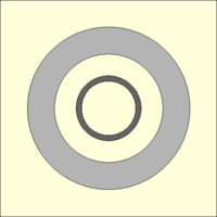
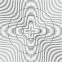
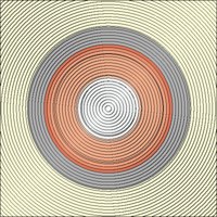
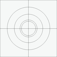
The test case is comprised of an isotropic, point-wise, low-energy neutron source, enclosed inside two cylindrical shells made of steel and concrete. The geometry is in 2D for the sake of simplicity, but the same procedures apply to 3D problems as well. The geometry plot and complete input listing are provided below (click Expand to show).
Completely made-up neutron shielding problem
 % --- Geometry (nested cylinders)

surf 1 cyl 0.0 0.0 100.0
surf 2 cyl 0.0 0.0 120.0
surf 3 cyl 0.0 0.0 200.0
surf 4 cyl 0.0 0.0 300.0
surf 5 sqc 0.0 0.0 400.0

cell 1 0 air      -1
cell 2 0 steel     1 -2
cell 3 0 air       2 -3
cell 4 0 concrete  3 -4
cell 5 0 air       4 -5
cell 6 0 outside   5

% --- Materials

mat steel    -8.00000E+00  rgb 100 100 100

 6000.03c    -4.00000E-04
14000.03c    -5.00000E-03
15031.03c    -2.30000E-04
16000.03c    -1.50000E-04
24000.03c    -1.90000E-01
25055.03c    -1.00000E-02
26000.03c    -7.01730E-01
28000.03c    -9.25000E-02

mat air      -1.20500E-03  rgb 255 255 220

 6000.03c    -1.24000E-04
 7014.03c    -7.55268E-01
 8016.03c    -2.31781E-01
18040.03c    -1.28270E-02

mat concrete -2.30000E+00  rgb 180 180 180

 1001.03c    -1.00000E-02
 8016.03c    -5.32000E-01
11023.03c    -2.90000E-02
13027.03c    -3.40000E-02
14000.03c    -3.37000E-01
20000.03c    -4.40000E-02
26000.03c    -1.40000E-02

% --- Source

src 1 sp 0 0 0 se 1E-6     % Isotropic 1 eV point source
set srcrate 1              % Normalize to unit source rate

% --- Run parameters

set nps 200000 50
set gcu -1                 % Group constant generation off

% --- Geometry plot:

plot 3 500 500

% --- Mesh plot (flux)

det F1                     % Flux detector
mesh 8 -4 F1 3 500 500     % Plot detector scores

% --- Detectors

det d1 dc 3                % Flux in airspace between walls

surf s2 cyl 0.0 160.0 5.0
det d2 dtl s2              % Flux at y = 160 (between the walls)

surf s3 cyl 0.0 350.0 5.0
det d3 dtl s3              % Flux at y = 350 (outside the concrete wall)
Notes on the input:
- Group constant generation is on by default in neutron transport simulations. This is switched off by set gcu -1.
- Neutron transport simulations are normalized by default to unit loss rate. For consistency the normalization is changed to unit source rate by set srcrate 1.
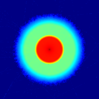
- The mesh-card is linked to a flux detector (type 8) to visualize the effect of variance reduction. The color scheme is set to logarithmic (negative entry). It should be noted that the normalization of the color scheme depends on the minimum and maximum values, so the plots produced with and without variance reduction are not similarly normalized.
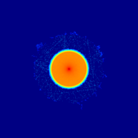
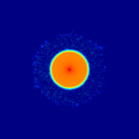
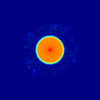
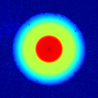
In addition to the mesh plot, flux is also calculated using a cell flux detector in the airspace between the walls (d1) and two track-length detectors at a position between the walls (d2) and outside the outer concrete wall (d3). The mesh plot and detector results are presented below (click image for full-size).
| Detector | Score | Relative statistical error |
|---|---|---|
| d1 (volume flux between shells) | 1.59600E-01 | 0.16735 |
| d2 (at y = 160) | 1.04553E-04 | 0.73813 |
| d3 (at y = 350) | 0.00000E+00 | 0.00000 |
The results show that most neutrons are stopped by the inner shell, and none of the particles are able to penetrate the concrete.
Variance reduction, simple approach
The simplest approach to applying variance reduction is to divide the calculation in two parts. The first run generates the importance mesh, and the second run produces the final results by applying the weight-window technique. The weigh window generator is invoked by adding the wgen card:
Complete input
 % --- Geometry (nested cylinders)

surf 1 cyl 0.0 0.0 100.0
surf 2 cyl 0.0 0.0 120.0
surf 3 cyl 0.0 0.0 200.0
surf 4 cyl 0.0 0.0 300.0
surf 5 sqc 0.0 0.0 400.0

cell 1 0 air      -1
cell 2 0 steel     1 -2
cell 3 0 air       2 -3
cell 4 0 concrete  3 -4
cell 5 0 air       4 -5
cell 6 0 outside   5

% --- Materials

mat steel    -8.00000E+00  rgb 100 100 100

 6000.03c    -4.00000E-04
14000.03c    -5.00000E-03
15031.03c    -2.30000E-04
16000.03c    -1.50000E-04
24000.03c    -1.90000E-01
25055.03c    -1.00000E-02
26000.03c    -7.01730E-01
28000.03c    -9.25000E-02

mat air      -1.20500E-03  rgb 255 255 220

 6000.03c    -1.24000E-04
 7014.03c    -7.55268E-01
 8016.03c    -2.31781E-01
18040.03c    -1.28270E-02

mat concrete -2.30000E+00  rgb 180 180 180

 1001.03c    -1.00000E-02
 8016.03c    -5.32000E-01
11023.03c    -2.90000E-02
13027.03c    -3.40000E-02
14000.03c    -3.37000E-01
20000.03c    -4.40000E-02
26000.03c    -1.40000E-02

% --- Source

src 1 sp 0 0 0 se 1E-6     % Isotropic 1 eV point source
set srcrate 1              % Normalize to unit source rate

% --- Run parameters

set nps 200000 50
set gcu -1                 % Group constant generation off

% --- Geometry plot:

plot 3 500 500

% --- Mesh plot (flux)

det F1                     % Flux detector
mesh 8 -4 F1 3 500 500     % Plot detector scores

% --- Detectors

det d1 dc 3                % Flux in airspace between walls

surf s2 cyl 0.0 160.0 5.0
det d2 dtl s2              % Flux at y = 160 (between the walls)

surf s3 cyl 0.0 350.0 5.0
det d3 dtl s3              % Flux at y = 350 (outside the concrete wall)

% --- Weight window generation

wwgen 1                    % wwgen identifier
1E-9 10000                 % convergence criteria
1 -1                       % single detector, no energy binning
1                          % Cartesian mesh
-400.01 400.01 51          % x-dimensions
-400.01 400.01 51          % y-dimensions
-1E18 1E18 1               % z-dimensions
d2 1.0                     % detecor name and weight factor
Notes:
- The geometry is covered by a Cartesian 51x51x1 mesh.
- An uneven number of cells is selected to prevent the point source (at origin) coinciding with the mesh boundaries.
- The mesh should be slightly larger (here 0.01 cm) than the geometry to prevent problems with numerical precision.
- In 2D calculations the axial limits should be set to large values to prevent particles escaping the mesh.
- The importances are calculated with respect to detector d2, positioned between the two shells.
When Serpent is run, the run-time output shows some information on the response matrix solution:
If the solution does not converge, the reason is most likely poor statistics.
The calculation produces a binary weight-window mesh file: [input].wwd, which can be read into another simulation using the wwin card:
Complete input
% --- Geometry (nested cylinders)

surf 1 cyl 0.0 0.0 100.0
surf 2 cyl 0.0 0.0 120.0
surf 3 cyl 0.0 0.0 200.0
surf 4 cyl 0.0 0.0 300.0
surf 5 sqc 0.0 0.0 400.0

cell 1 0 air      -1
cell 2 0 steel     1 -2
cell 3 0 air       2 -3
cell 4 0 concrete  3 -4
cell 5 0 air       4 -5
cell 6 0 outside   5

% --- Materials

mat steel    -8.00000E+00  rgb 100 100 100

 6000.03c    -4.00000E-04
14000.03c    -5.00000E-03
15031.03c    -2.30000E-04
16000.03c    -1.50000E-04
24000.03c    -1.90000E-01
25055.03c    -1.00000E-02
26000.03c    -7.01730E-01
28000.03c    -9.25000E-02

mat air      -1.20500E-03  rgb 255 255 220

 6000.03c    -1.24000E-04
 7014.03c    -7.55268E-01
 8016.03c    -2.31781E-01
18040.03c    -1.28270E-02

mat concrete -2.30000E+00  rgb 180 180 180

 1001.03c    -1.00000E-02
 8016.03c    -5.32000E-01
11023.03c    -2.90000E-02
13027.03c    -3.40000E-02
14000.03c    -3.37000E-01
20000.03c    -4.40000E-02
26000.03c    -1.40000E-02

% --- Source

src 1 sp 0 0 0 se 1E-6     % Isotropic 1 eV point source
set srcrate 1              % Normalize to unit source rate

% --- Run parameters

set nps 200000 50
set gcu -1                 % Group constant generation off
set bala 1                 % Use OMP load balancing

% --- Geometry plot:

plot 35 1E-4 1E4 -1 500 500

% --- Mesh plot (flux)

det F1                     % Flux detector
mesh 8 -4 F1 3 500 500     % Plot detector scores

% --- Detectors

det d1 dc 3                % Flux in airspace between walls

surf s2 cyl 0.0 160.0 5.0
det d2 dtl s2              % Flux at y = 160 (between the walls)

surf s3 cyl 0.0 350.0 5.0
det d3 dtl s3              % Flux at y = 350 (outside the concrete wall)

% --- Weight windows

wwin 1 wf "YOUR_FILE.wwd" 1     % Read from previous run
Notes on the input:
- Variance reduction causes splitting of the particle histories, which may result in deterioration of OpenMP parallel scalability. To improve performance, it is recommended to switch OpenMP load balancing on by set bala 1.
- The importance mesh can be plotted on top of the geometry using the plot card. The additional input parameters include importance boundaries and energy (for energy-dependent calculations).
- The current version of Serpent (2.1.31) does not plot the mesh grid for the importance distribution, but this can be enabled by removing the "wwp = NO;" statement on line 116 of geometryplotter.c
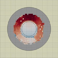
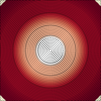
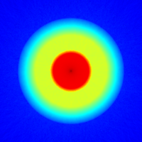
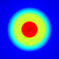
The mesh plot and detector results using variance reduction are presented below (click image for full-size).
| Detector | Score | Relative statistical error |
|---|---|---|
| d1 (volume flux between shells) | 1.18215E-01 | 0.14545 |
| d2 (at y = 160) | 1.50203E-04 | 0.10000 |
| d3 (at y = 350) | 0.00000E+00 | 0.00000 |
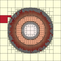
The importances were calculated with respect to detector d2, which recieves much better statistics compared to the analog calculation. The mesh plot shows how the calculated flux is concentrated around the detectors, as particles less likely to contribute to the result are killed by Russian roulette.
Global variance reduction, fixed mesh
One of the challenges with large and heavily shielded geometries is that the particle histories may not reach the region of interest, in which case the Monte Carlo simulation fails to provide the coupling coefficients for the response matrix method-based importance solver. The solution is to apply global variance reduction (GVR), which means producing a weight-window mesh that uniformly populates the entire geometry. The calculation proceeds by iterations. Each cycle allows the particles to wonder beyond the region charted for the weight-window mesh, and the collected new data is used to extend the mesh deeper into the geometry.
This option is invoked by setting the MOD parameter to 3 in the wgen card. Also the detector entry is left out. The mesh type is changed to cylindrical. In this example global variance reduction is used with weight window iterations. The input is listed below.
Complete input
% --- Geometry (nested cylinders)

surf 1 cyl 0.0 0.0 100.0
surf 2 cyl 0.0 0.0 120.0
surf 3 cyl 0.0 0.0 200.0
surf 4 cyl 0.0 0.0 300.0
surf 5 sqc 0.0 0.0 400.0

cell 1 0 air      -1
cell 2 0 steel     1 -2
cell 3 0 air       2 -3
cell 4 0 concrete  3 -4
cell 5 0 air       4 -5
cell 6 0 outside   5

% --- Materials

mat steel    -8.00000E+00  rgb 100 100 100

 6000.03c    -4.00000E-04
14000.03c    -5.00000E-03
15031.03c    -2.30000E-04
16000.03c    -1.50000E-04
24000.03c    -1.90000E-01
25055.03c    -1.00000E-02
26000.03c    -7.01730E-01
28000.03c    -9.25000E-02

mat air      -1.20500E-03  rgb 255 255 220

 6000.03c    -1.24000E-04
 7014.03c    -7.55268E-01
 8016.03c    -2.31781E-01
18040.03c    -1.28270E-02

mat concrete -2.30000E+00  rgb 180 180 180

 1001.03c    -1.00000E-02
 8016.03c    -5.32000E-01
11023.03c    -2.90000E-02
13027.03c    -3.40000E-02
14000.03c    -3.37000E-01
20000.03c    -4.40000E-02
26000.03c    -1.40000E-02

% --- Source

src 1 sp 0 0 0 se 1E-6     % Isotropic 1 eV point source
set srcrate 1              % Normalize to unit source rate

% --- Run parameters

set nps 200000 50
set gcu -1                 % Group constant generation off
set bala 1                 % Use OMP load balancing

% --- Geometry plot:

plot 35 1E-9 1E9 -1 500 500

% --- Mesh plot (flux)

det F1                     % Flux detector
mesh 8 -4 F1 3 500 500     % Plot detector scores

% --- Detectors

det d1 dc 3                % Flux in airspace between walls

surf s2 cyl 0.0 160.0 5.0
det d2 dtl s2              % Flux at y = 160 (between the walls)

surf s3 cyl 0.0 350.0 5.0
det d3 dtl s3              % Flux at y = 350 (outside the concrete wall)

% --- Weight window generation

wwgen 1                    % wwgen identifier
1E-9 10000                 % convergence criteria
3 -1                       % global variance reduction, no energy binning
2                          % cylindrical mesh
0.0 565.70 50              % radial dimensions
0.0 360.00 1               % azimuthal dimensions
-1E18 1E18 1               % axial dimensions

% --- GVR iterations

wwin 1
wi 1 3                     % 3 iterations using the same mesh
1 1.0
1 1.0
1 1.0
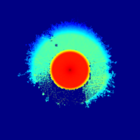
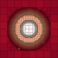
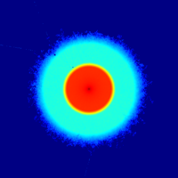
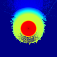
The geometry and mesh plots and detector results are presented below.
| Detector | Score | Relative statistical error |
|---|---|---|
| d1 (volume flux between shells) | 1.67545E-01 | 0.02275 |
| d2 (at y = 160) | 1.48163E-04 | 0.05940 |
| d3 (at y = 350) | 4.51737E-10 | 0.09170 |
The GVR iterations push particle population through the shielded parts of the geometry, resulting in non-zero statistics olso for the outermost detector.
Global variance reduction, adaptive mesh
The most elaborate solution to deep penetration problems is to first run GVR iterations until the region of interest is populated, and then produce the optimal weight-window mesh for the detector. In practice this involves three runs:
- GVR iteration until the geometry is sufficiently populated
- Generation of the optimal weight-window mesh
- Final transport simulation using the optimal mesh.
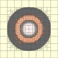
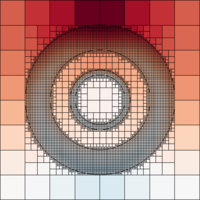
This approach is demonstrated using the adaptive mesh option. A coarse Cartesian base mesh is laid on top of the geometry, and the cells are recursively split to adapt the mesh around the dense parts of the geometry. The input is listed below.
Complete input
% --- Geometry (nested cylinders)

surf 1 cyl 0.0 0.0 100.0
surf 2 cyl 0.0 0.0 120.0
surf 3 cyl 0.0 0.0 200.0
surf 4 cyl 0.0 0.0 300.0
surf 5 sqc 0.0 0.0 400.0

cell 1 0 air      -1
cell 2 0 steel     1 -2
cell 3 0 air       2 -3
cell 4 0 concrete  3 -4
cell 5 0 air       4 -5
cell 6 0 outside   5

% --- Materials

mat steel    -8.00000E+00  rgb 100 100 100

 6000.03c    -4.00000E-04
14000.03c    -5.00000E-03
15031.03c    -2.30000E-04
16000.03c    -1.50000E-04
24000.03c    -1.90000E-01
25055.03c    -1.00000E-02
26000.03c    -7.01730E-01
28000.03c    -9.25000E-02

mat air      -1.20500E-03  rgb 255 255 220

 6000.03c    -1.24000E-04
 7014.03c    -7.55268E-01
 8016.03c    -2.31781E-01
18040.03c    -1.28270E-02

mat concrete -2.30000E+00  rgb 180 180 180

 1001.03c    -1.00000E-02
 8016.03c    -5.32000E-01
11023.03c    -2.90000E-02
13027.03c    -3.40000E-02
14000.03c    -3.37000E-01
20000.03c    -4.40000E-02
26000.03c    -1.40000E-02

% --- Source

src 1 sp 0 0 0 se 1E-6     % Isotropic 1 eV point source
set srcrate 1              % Normalize to unit source rate

% --- Run parameters

set nps 200000 50
set gcu -1                 % Group constant generation off
set bala 1                 % Use OMP load balancing

% --- Geometry plot:

plot 35 1E-9 1E9 -1 500 500

% --- Mesh plot (flux)

det F1                     % Flux detector
mesh 8 -4 F1 3 500 500     % Plot detector scores

% --- Detectors

det d1 dc 3                % Flux in airspace between walls

surf s2 cyl 0.0 160.0 5.0
det d2 dtl s2              % Flux at y = 160 (between the walls)

surf s3 cyl 0.0 350.0 5.0
det d3 dtl s3              % Flux at y = 350 (outside the concrete wall)

% --- Weight window generation

wwgen 1                    % wwgen identifier
1E-9 10000                 % convergence criteria
3 -1                       % global variance reduction, no energy binning
1                          % cartesian mesh
-400.01 400.01 2           % x-dimensions
-400.01 400.01 2           % y-dimensions
-1E18 1E18 1               % z-dimensions

% --- Generation of Adaptive mesh and iterations

wwin 1
wi 2 4 1                   % run 4 iterations with adaptive mesh
2 2 1                      % split cells in half (x and y only)
10 2000                    % 10 outer iterations 2000 tracks
1E9 1000000                % importance and neighbor criteria
-1.0 5.0 5.0 5.0           % density criteria and minimum dimensions
Notes on the input:
- The adaptive mesh is generated based on split and stop criteria.
- When split, the cells are divided into 2x2x1 new cells (2D geometry, no splitting in z).
- In this example the splits are based on the density criterion only. The importance and neighbor criteria are eliminated by using high limits.
- Splitting occurs if the cell contains a dense material (density above 1.0 g/cm3), unless the size is already below the minimum (5x5x5 cm).
The geometry and mesh plots and detector results are presented below.
| Detector | Score | Relative statistical error |
|---|---|---|
| d1 (volume flux between shells) | 1.64883E-01 | 0.01643 |
| d2 (at y = 160) | 1.55702E-04 | 0.02679 |
| d3 (at y = 350) | 4.30948E-10 | 0.05926 |
The GVR iterations produce 4 weight window files [input].wwd0 ... [input].wwd3. The last mesh is next used for variance reduction in the next simulation, in which the weight-window mesh is optimized for detector d3:
Complete input
% --- Geometry (nested cylinders)

surf 1 cyl 0.0 0.0 100.0
surf 2 cyl 0.0 0.0 120.0
surf 3 cyl 0.0 0.0 200.0
surf 4 cyl 0.0 0.0 300.0
surf 5 sqc 0.0 0.0 400.0

cell 1 0 air      -1
cell 2 0 steel     1 -2
cell 3 0 air       2 -3
cell 4 0 concrete  3 -4
cell 5 0 air       4 -5
cell 6 0 outside   5

% --- Materials

mat steel    -8.00000E+00  rgb 100 100 100

 6000.03c    -4.00000E-04
14000.03c    -5.00000E-03
15031.03c    -2.30000E-04
16000.03c    -1.50000E-04
24000.03c    -1.90000E-01
25055.03c    -1.00000E-02
26000.03c    -7.01730E-01
28000.03c    -9.25000E-02

mat air      -1.20500E-03  rgb 255 255 220

 6000.03c    -1.24000E-04
 7014.03c    -7.55268E-01
 8016.03c    -2.31781E-01
18040.03c    -1.28270E-02

mat concrete -2.30000E+00  rgb 180 180 180

 1001.03c    -1.00000E-02
 8016.03c    -5.32000E-01
11023.03c    -2.90000E-02
13027.03c    -3.40000E-02
14000.03c    -3.37000E-01
20000.03c    -4.40000E-02
26000.03c    -1.40000E-02

% --- Source

src 1 sp 0 0 0 se 1E-6     % Isotropic 1 eV point source
set srcrate 1              % Normalize to unit source rate

% --- Run parameters

set nps 200000 50
set gcu -1                 % Group constant generation off
set bala 1                 % Use OMP load balancing

% --- Geometry plot:

plot 35 1E-9 1E9 -1 500 500

% --- Mesh plot (flux)

det F1                     % Flux detector
mesh 8 -4 F1 3 500 500     % Plot detector scores

% --- Detectors

det d1 dc 3                % Flux in airspace between walls

surf s2 cyl 0.0 160.0 5.0
det d2 dtl s2              % Flux at y = 160 (between the walls)

surf s3 cyl 0.0 350.0 5.0
det d3 dtl s3              % Flux at y = 350 (outside the concrete wall)

% --- Weight window generation

wwgen 1                    % wwgen identifier
1E-9 10000                 % convergence criteria
1 -1                       % single detector, no energy binning
-1                         % use mesh from file
d3 1.0

% --- Weight windows

wwin 1
wf "YOUR_FILE1.wwd3" 1           % read last mesh from previous iteration
Notes:
- The mesh type in the wgen card must be set to -1 when the mesh is read from a file.
- The type is again set to 1 (single detector) and the detector entry added at the end.
The result is a final weight-window mesh file, optimized for detector d3. This mesh is read into the third input:
Complete input
% --- Geometry (nested cylinders)

surf 1 cyl 0.0 0.0 100.0
surf 2 cyl 0.0 0.0 120.0
surf 3 cyl 0.0 0.0 200.0
surf 4 cyl 0.0 0.0 300.0
surf 5 sqc 0.0 0.0 400.0

cell 1 0 air      -1
cell 2 0 steel     1 -2
cell 3 0 air       2 -3
cell 4 0 concrete  3 -4
cell 5 0 air       4 -5
cell 6 0 outside   5

% --- Materials

mat steel    -8.00000E+00  rgb 100 100 100

 6000.03c    -4.00000E-04
14000.03c    -5.00000E-03
15031.03c    -2.30000E-04
16000.03c    -1.50000E-04
24000.03c    -1.90000E-01
25055.03c    -1.00000E-02
26000.03c    -7.01730E-01
28000.03c    -9.25000E-02

mat air      -1.20500E-03  rgb 255 255 220

 6000.03c    -1.24000E-04
 7014.03c    -7.55268E-01
 8016.03c    -2.31781E-01
18040.03c    -1.28270E-02

mat concrete -2.30000E+00  rgb 180 180 180

 1001.03c    -1.00000E-02
 8016.03c    -5.32000E-01
11023.03c    -2.90000E-02
13027.03c    -3.40000E-02
14000.03c    -3.37000E-01
20000.03c    -4.40000E-02
26000.03c    -1.40000E-02

% --- Source

src 1 sp 0 0 0 se 1E-6     % Isotropic 1 eV point source
set srcrate 1              % Normalize to unit source rate

% --- Run parameters

set nps 200000 50
set gcu -1                 % Group constant generation off
set bala 1                 % Use OMP load balancing

% --- Geometry plot:

plot 35 1E-9 1E9 -1 500 500

% --- Mesh plot (flux)

det F1                     % Flux detector
mesh 8 -4 F1 3 500 500     % Plot detector scores

% --- Detectors

det d1 dc 3                % Flux in airspace between walls

surf s2 cyl 0.0 160.0 5.0
det d2 dtl s2              % Flux at y = 160 (between the walls)

surf s3 cyl 0.0 350.0 5.0
det d3 dtl s3              % Flux at y = 350 (outside the concrete wall)

% --- Weight windows

wwin 1
wf "YOUR_FILE2.wwd" 1
The geometry and mesh plots and detector results are presented below.
| Detector | Score | Relative statistical error |
|---|---|---|
| d1 (volume flux between shells) | 1.73844E-01 | 0.08012 |
| d2 (at y = 160) | 1.61522E-04 | 0.02736 |
| d3 (at y = 350) | 4.64133E-10 | 0.03110 |
References
- ^ Lux, I. and Koblinger, L. "Monte Carlo Particle Transport Methods: Neutron and Photon Calculations." CRC-Press, 1991. (available on-line).
- ^ D. Pelowitz (ed.), “MCNP6 User’s Manual: Appendix C Mesh-Based WWINP, WWOUT, and WWONE File Format,” LA-CP-13-00634, Los Alamos National Laboratory (2013).
- ^ J. Leppänen "Response Matrix Method–Based Importance Solver and Variance Reduction Scheme in the Serpent 2 Monte Carlo Code." Nucl. Technol. (in press)
- ^ J. Leppänen and M. Jokipii. "Global Variance Reduction Scheme with Self-Adaptive Weight-Window Mesh in the Serpent 2 Monte Carlo Code." In Proc. M&C2019, Portland, OR, Aug. 25-29, 2019.
