Difference between revisions of "Flattop k-eff sensitivity example"
(→Results) |
Ana Jambrina (talk | contribs) (→Input) |
||
| (11 intermediate revisions by 3 users not shown) | |||
| Line 1: | Line 1: | ||
| − | This example demonstrates some basic sensitivity calculation capabilities for the Popsy (Flattop) critical experiment (PU-MET-FAST-006 in the ICSBEP handbook). | + | This example demonstrates some basic [[Sensitivity calculations|sensitivity calculation capabilities]] for the Popsy (Flattop) critical experiment (PU-MET-FAST-006 in the ICSBEP handbook). |
== Description == | == Description == | ||
| Line 43: | Line 43: | ||
set pop 10000 100000 50 1 100 100 | set pop 10000 100000 50 1 100 100 | ||
| + | |||
| + | % --- Use a central point source as the initial source | ||
| + | |||
| + | src point sp 0.0 0.0 0.0 | ||
% --- Write output each 100 cycles | % --- Write output each 100 cycles | ||
| Line 54: | Line 58: | ||
% --- Use unresolved resonance sampling for the fast system | % --- Use unresolved resonance sampling for the fast system | ||
| − | set ures 1 | + | set ures 1 |
% --- Define Vitamin-J energy grid (one of the defaults) | % --- Define Vitamin-J energy grid (one of the defaults) | ||
| Line 96: | Line 100: | ||
sens pert matlist total | sens pert matlist total | ||
| − | % --- Perturb cross sections separately for each | + | % --- Perturb cross sections separately for each sum reaction mode (fission, capture etc.) |
sens pert xs all | sens pert xs all | ||
| Line 215: | Line 219: | ||
%% --- Run the sensitivity output file | %% --- Run the sensitivity output file | ||
| − | run([fname ' | + | run([fname '_sens0.m']); |
%% --- Print some basic output data | %% --- Print some basic output data | ||
| Line 391: | Line 395: | ||
end | end | ||
end</nowiki> | end</nowiki> | ||
| + | </div> | ||
| + | </div> | ||
| + | |||
| + | === Scripts for visualizing with Python === | ||
| + | |||
| + | The following two scripts rely on the serpentTools python package for the parsing of the output | ||
| + | and plotting https://serpent-tools.readthedocs.io/en/latest/ | ||
| + | |||
| + | Fonts are configured with matplotlib to look like LaTeX | ||
| + | https://matplotlib.org/tutorials/introductory/customizing.html | ||
| + | |||
| + | Full example of the sensitivity reader can be found at | ||
| + | https://serpent-tools.readthedocs.io/en/latest/examples/Sensitivity.html | ||
| + | |||
| + | <div class="toccolours mw-collapsible mw-collapsed" style="width:80em;"> | ||
| + | '''Simple python processing script:''' | ||
| + | <div class="mw-collapsible-content"> | ||
| + | |||
| + | <pre>"""Script for visualizing k-eff sensitivities for Flattop problem""" | ||
| + | from matplotlib import pyplot | ||
| + | import serpentTools | ||
| + | |||
| + | s = serpentTools.read("flattop_sens.m") | ||
| + | |||
| + | # Only response is required, but then it plots against all | ||
| + | # permutations of materials, perturbations, and materials | ||
| + | # Pass material and/or isotope ZAI and/or specific perturbation to plot | ||
| + | # sensitivities due to those properties only | ||
| + | # s.plot handles log scaling, step plotting, and uncertainty | ||
| + | |||
| + | s.plot( | ||
| + | "keff", mat="total", zai=922380, pert="fission xs", | ||
| + | ) | ||
| + | |||
| + | # Format the plot to look like the MATLAB / OCTAVE example | ||
| + | # No y axis limits | ||
| + | |||
| + | pyplot.xlim(1E4, s.energies[-1]*1E6) | ||
| + | |||
| + | # Turn on minor grids for the x-axis to show the log scale better | ||
| + | pyplot.grid("x", which="both") | ||
| + | pyplot.grid("y") | ||
| + | |||
| + | # Add a title to the top of the figure | ||
| + | pyplot.title("Response: K-eff Material: total ZAI: 922380 perturbation: fission xs") | ||
| + | |||
| + | # Show the figure | ||
| + | pyplot.show() | ||
| + | </pre> | ||
| + | </div> | ||
| + | </div> | ||
| + | |||
| + | <div class="toccolours mw-collapsible mw-collapsed" style="width:80em;"> | ||
| + | '''Detailed python processing script:''' | ||
| + | <div class="mw-collapsible-content"> | ||
| + | |||
| + | This script seeks to fully replicate the figures provided in the Wiki made using the MATLAB / OCTAVE | ||
| + | programs | ||
| + | |||
| + | <pre> | ||
| + | from matplotlib import pyplot | ||
| + | import serpentTools | ||
| + | |||
| + | s = serpentTools.read("flattop_sens.m") | ||
| + | |||
| + | # Extract the response of interest from the sensitivities dictionary | ||
| + | |||
| + | ks = s.sensitivities["keff"] | ||
| + | |||
| + | # Obtain the expected value and uncertainty by indexing into the multi-dimensional | ||
| + | # response. The matrix is structured [materials, isotopes, perturbations, energies, 2] | ||
| + | # where the last dimension stores value and uncertainty | ||
| + | # We can use the materials, zais, and perts dictionaries to obtain the correct index | ||
| + | # in each dimension for the quantity of interest | ||
| + | |||
| + | kslice = ks[ | ||
| + | s.materials["total"], # index for sensitivity due to all materials | ||
| + | s.zais[922380], # index for sensitivity due to U238 | ||
| + | s.perts["fission xs"], # index for sensitivity due to fission xs | ||
| + | ] | ||
| + | |||
| + | # Normalize per unit lethargy | ||
| + | # Python arrays are zero-indexed, so the expected value is in the 0 index | ||
| + | value = kslice[:, 0] / s.lethargyWidths | ||
| + | |||
| + | # Compute 2-sigma uncertainty | ||
| + | unc = kslice[:, 1] * 2 * value | ||
| + | |||
| + | # Draw errorbars | ||
| + | # The energy vector has one additional entry, so we will instead drop the first item | ||
| + | # by slicing from the second position forward | ||
| + | pyplot.errorbar( | ||
| + | s.energies[1:] * 1E6, # convert to MeV | ||
| + | value, # expected value | ||
| + | yerr=unc, # uncertainty | ||
| + | drawstyle="steps-mid", # step-plot | ||
| + | c="k", # draw using a black line | ||
| + | ) | ||
| + | |||
| + | # Shade the region under the curve red | ||
| + | # Use a mild transparency | ||
| + | pyplot.fill_between(s.energies[1:]*1E6, value, color="tab:red", alpha=0.3, step="mid") | ||
| + | |||
| + | # Format the plot | ||
| + | pyplot.xscale("log") | ||
| + | pyplot.xlim(1E4, s.energies[-1]*1E6) | ||
| + | # Major and minor grids for the log-scaled x axis | ||
| + | pyplot.grid("x", which="both") | ||
| + | pyplot.grid("y") | ||
| + | pyplot.xlabel("Energy (eV)") | ||
| + | pyplot.ylabel("Sensitivity per unit lethargy") | ||
| + | pyplot.title("Response: K-eff Material: total ZAI: 922380 perturbation: fission xs") | ||
| + | |||
| + | pyplot.show() | ||
| + | </pre> | ||
</div> | </div> | ||
</div> | </div> | ||
| Line 469: | Line 588: | ||
These results were obtained using ENDF/B-VII.1 based cross section libraries. | These results were obtained using ENDF/B-VII.1 based cross section libraries. | ||
| + | |||
| + | A number of produced figures are also shown here for ease of comparison: | ||
| + | |||
| + | [[File:Popsy_sensitivity_K-eff_sens_1_4_6.png|thumb|left|700px|Sensitivity profile of k-eff to perturbation of <sup>239</sup>Pu fission cross section.]] | ||
| + | [[File:Popsy_sensitivity_K-eff_sens_1_3_6.png|thumb|left|700px|Sensitivity profile of k-eff to perturbation of <sup>238</sup>U fission cross section.]] | ||
| + | [[File:Popsy_sensitivity_K-eff_sens_1_3_2.png|thumb|left|700px|Sensitivity profile of k-eff to perturbation of <sup>238</sup>U elastic scattering cross section.]] | ||
| + | |||
| + | [[File:Popsy_sensitivity_K-eff_sens_python_short.png|thumb|left|700px|Sensitivity profile of k-eff to perturbation of <sup>238</sup>U fission cross section. Generated with simple python script]] | ||
| + | [[File:Popsy_sensitivity_K-eff_sens_python_handmade.png|thumb|left|700px|Sensitivity profile of k-eff to perturbation of <sup>238</sup>U fission cross section. Generated with detailed python script]] | ||
| + | |||
| + | [[Category:Example input files]] | ||
Latest revision as of 14:54, 5 June 2022
This example demonstrates some basic sensitivity calculation capabilities for the Popsy (Flattop) critical experiment (PU-MET-FAST-006 in the ICSBEP handbook).
Contents
Description
The experimental configuration consists of a plutonium alloy sphere (radius 4.5332 cm) reflected by a natural uranium blanket (outer radius 24.1420 cm). The multiplication factor of the system is close to unity (being a critical experiment). This input calculates the sensitivity of the multiplication factor to perturbations applied to the cross sections of 235U, 238U, 239Pu and 240Pu. A processing script for MATLAB/OCTAVE is provided for printing and plotting out the sensitivities.
Input
Input for Popsy (Flattop) sensitivity calculation example:
% --- Core outer surface and blanket outer surface

surf s1 sph 0.0 0.0 0.0  4.5332
surf s2 sph 0.0 0.0 0.0 24.1420

% --- Divide space to core, blanket and outside

cell c1 0 core       -s1
cell c3 0 blanket s1 -s2
cell c4 0 outside s2

% --- Core is made from plutonium alloy

mat core sum
94239.03c  3.6697e-2
94240.03c  1.8700e-3
94241.03c  1.1639e-4
31000.03c  1.4755e-3

% --- Blanket is made from natural uranium

mat blanket sum
92234.03c  2.6438e-6
92235.03c  3.4610e-4
92238.03c  4.7721e-2

% --- Cross section libraries

%set acelib "<path-to-acelib>"

% --- Neutron population

set pop 10000 100000 50 1 100 100

% --- Use a central point source as the initial source

src point sp 0.0 0.0 0.0

% --- Write output each 100 cycles

set outp 100

% --- Modify event buffer size to 3 events per neutron

set nbuf 3 3

% --- Use unresolved resonance sampling for the fast system

set ures 1

% --- Define Vitamin-J energy grid (one of the defaults)

ene myvit-j 4 nj23

% %%%
% %%% --- Sensitivity options
% %%%

% --- Run sensitivity calculation using Vitamin-J energy grid

sens opt egrid myvit-j

% --- Use 15 latent generations for the sensitivity calculations

sens opt latgen 15

% --- Use 10 generations for Iterated Fission Probability

set ifp 10

% %%%
% %%% --- Sensitivity responses
% %%%

% --- Calculate sensitivity of k-effective to perturbations

sens resp keff

% %%%
% %%% --- Sensitivity perturbations
% %%%

% --- Separate perturbations for the different nuclides and total

sens pert zailist 922350 922380 942390 942400 total

% --- Do not calculate material-wise perturbations (only total)

sens pert matlist total

% --- Perturb cross sections separately for each sum reaction mode (fission, capture etc.)

sens pert xs all

% --- Score sensitivity results directly to a matrix for each particle
%     Assume 0.2 matrices needed per generation per particle

sens opt direct 0.2
Output
The contents of some long arrays have been replaced with "...".
Output for Popsy (Flattop) sensitivity calculation example:
% Number of different bins in sensitivity calculation:

SENS_N_MAT = 1;
SENS_N_ZAI = 5;
SENS_N_PERT = 7;
SENS_N_ENE = 175;

% Materials included in sensitivity calculation:

SENS_MAT_LIST = [
'total               '
];

% Indices for different materials:

iSENS_MAT_TOT              = 1;

% Nuclides included in sensitivity calculation:

SENS_ZAI_LIST = [
0        % total
922350
922380
942390
942400
];

% Indices for different ZAIs:

iSENS_ZAI_TOT	   = 1;
iSENS_ZAI_922350   = 2;
iSENS_ZAI_922380   = 3;
iSENS_ZAI_942390   = 4;
iSENS_ZAI_942400   = 5;

% Reactions included in sensitivity calculation:

SENS_PERT_LIST = [
'total xs            '
'ela scatt xs        '
'sab scatt xs        '
'inl scatt xs        '
'capture xs          '
'fission xs          '
'nxn xs              '
];

% Indices for different perturbations:

iSENS_PERT_TOT_XS	= 1;
iSENS_PERT_ELA_XS	= 2;
iSENS_PERT_SAB_XS	= 3;
iSENS_PERT_INL_XS	= 4;
iSENS_PERT_CAPT_XS	= 5;
iSENS_PERT_FISS_XS	= 6;
iSENS_PERT_NXN_XS	= 7;

% Sensitivity calculation energy group boundaries:

SENS_E = [  ...  ];

% Sensitivity calculation energy group lethargy widths:

SENS_LETHARGY_WIDTHS = [  ...  ];

% Sensitivities with 15 latent generations:

% Effective multiplication factor:

ADJ_PERT_KEFF_SENS = [
  ...
];

ADJ_PERT_KEFF_SENS = reshape(ADJ_PERT_KEFF_SENS, [2, SENS_N_ENE, SENS_N_PERT, SENS_N_ZAI, SENS_N_MAT]);
ADJ_PERT_KEFF_SENS = permute(ADJ_PERT_KEFF_SENS, [5, 4, 3, 2, 1]);

ADJ_PERT_KEFF_SENS_E_INT = [
  ...
];

ADJ_PERT_KEFF_SENS_E_INT = reshape(ADJ_PERT_KEFF_SENS_E_INT, [2, SENS_N_PERT, SENS_N_ZAI, SENS_N_MAT]);
ADJ_PERT_KEFF_SENS_E_INT = permute(ADJ_PERT_KEFF_SENS_E_INT, [4, 3, 2, 1]);
Data-processing and plotting
Script for printing and plotting the results tested with MATLAB R2014a and OCTAVE 4.0.0:
%% --- Flag to print out zero values

printzeros = false;

%% --- Input file name

fname = 'input';

%% --- Run the sensitivity output file

run([fname '_sens0.m']);

%% --- Print some basic output data

disp(sprintf('Results from Serpent sensitivity calculation using:\n'));

%% --- Materials

disp([num2str(SENS_N_MAT) ' perturbed materials:']);

for i=1:1:SENS_N_MAT
  disp(SENS_MAT_LIST(i,:));
end

%% --- Nuclides

disp(sprintf(['\n' num2str(SENS_N_ZAI) ' perturbed nuclides (ZAIs):']));

for i=1:1:SENS_N_ZAI
  disp(sprintf('%d',SENS_ZAI_LIST(i,:)));
end

%% --- Perturbations

disp(sprintf(['\n' num2str(SENS_N_PERT) ' different perturbations:']));

for i=1:1:SENS_N_PERT
  disp(SENS_PERT_LIST(i,:));
end

%% --- Energy grid

disp(sprintf(['\nEnergy grid with ' num2str(SENS_N_ENE) ' bins.']));

%%%%%%%%%%%%%%%%%%%%%%%%%%%%%%%%%%%%%%%%%%%%%%%%%%%%%%%%%%%%%%%
%% -- Output sensitivities one by one %%%%%%%%%%%%%%%%%%%%%%%%%
%%%%%%%%%%%%%%%%%%%%%%%%%%%%%%%%%%%%%%%%%%%%%%%%%%%%%%%%%%%%%%%

disp(sprintf('\n********************\n\nSensitivity results:\n'))

txt = sprintf('%-20s %-6s %-20s  : %12s | 2 sigma confidence interval', 'Material', 'ZAI', ' Perturbation', 'sensitivity');
disp(txt)

%% --- This script only prints/plots the k-eff sensitivities
%%     You can change the following three lines to plot something else

res  = ADJ_PERT_KEFF_SENS;
resE = ADJ_PERT_KEFF_SENS_E_INT;
resStr = 'K-eff';

for iMat=1:1:SENS_N_MAT

  matStr = SENS_MAT_LIST(iMat,:);

  for iZai=1:1:SENS_N_ZAI

    myZai = SENS_ZAI_LIST(iZai);

    %% --- Turn ZAI into a string for printing

    if (myZai == 0)
      zaiStr = sprintf('%-6s ', 'total');
    else
      zaiStr = sprintf('%6d ', SENS_ZAI_LIST(iZai));
    end

    %% --- Last loop is over perturbations

    for iPert=1:1:SENS_N_PERT

      %% --- Turn perturbation into a string for printing

      pertStr = sprintf('%-20s ', SENS_PERT_LIST(iPert,:));

      val = resE(iMat,iZai,iPert,1);
      err = resE(iMat,iZai,iPert,2);

      %% --- Calculate 2 sigma confidence interval assuming
      %%     normally distributed random variable

      minV = min([val*(1-2*err), val*(1+2*err)]);
      maxV = max([val*(1-2*err), val*(1+2*err)]);

      %% --- Create a formatted string for printing out the sensitivity

      txt = sprintf('%-20s %-6s %-20s: %+12.8f | [%+12.8f, %+12.8f]', matStr, zaiStr, pertStr, val, minV, maxV);

      %% --- Print formatted string

      if (printzeros || (val ~= 0) || (err ~= 0))
        disp(txt);

        %% --- Move on to plotting a stairstep plot

        %% --- Convert energy grid to eV

        xvals = SENS_E*1e6;

        %% --- Get energy dependent sensitivity and relative error

        yvals = squeeze(res(iMat, iZai, iPert, :, 1))./SENS_LETHARGY_WIDTHS';
        yerr = squeeze(res(iMat, iZai, iPert, :, 2));

        %% --- We'll need to re-append the last value if we want to
        %%     get the stairstep plot correct

        yvals = [yvals; yvals(end)];
        yerr = [yerr; yerr(end)];

        %% --- Create the figure for plotting

        fig1 = figure('visible', 'off');

        %% --- Plot the sample mean

        h1 = stairs(xvals, yvals, 'k-');
        set(h1, 'LineWidth', 2);

        %% --- Plot the sample mean +- 2*sqrt(sample variance)

        hold on;

        h2 = stairs(xvals, yvals.*(1+2*yerr), 'r-');
        h3 = stairs(xvals, yvals.*(1-2*yerr), 'r-');

        %% --- Fill the area of non-zero-sensitivity

        N = size(xvals,2)*2-2;
        xx = zeros(N,1);
        yy = zeros(N,1);

        xx(1:2:N) = xvals(1:1:end-1);
        xx(2:2:N) = xvals(2:1:end);
        yy(1:2:N) = yvals(1:1:end-1);
        yy(2:2:N) = yvals(1:1:end-1);

        h4 = fill(xx, yy, [1.0 0.8 0.8]);

        hold off;

        %% --- Make the picture a bit nicer

        set(gca,'xscale','log');
        set(gca,'XTick', [1e4 1e5 1e6 1e7]);

        grid on;
        box on;

        xlim([1e4, SENS_E(end)*1e6]);
        ylim([-0.1, 0.5]);

        %% --- Label the axes and add a title

        xlabel('Energy (eV)');
        ylabel('Sensitivity per unit lethargy');

        txt = sprintf('Response: %s\nMaterial: %s\nZAI: %s\n perturbation %s', resStr, matStr, zaiStr, pertStr);
        title(txt);

        %% --- Save the plot to file

        filename = sprintf('%s_sens_%ld_%ld_%ld.png', resStr, iMat, iZai, iPert);

        print(filename,'-dpng');

        %% --- Close figure
        close(fig1);

      end

    end
    %% --- Add empty line after each ZAI

    disp(sprintf(' '));
  end
end
Scripts for visualizing with Python
The following two scripts rely on the serpentTools python package for the parsing of the output and plotting https://serpent-tools.readthedocs.io/en/latest/
Fonts are configured with matplotlib to look like LaTeX https://matplotlib.org/tutorials/introductory/customizing.html
Full example of the sensitivity reader can be found at https://serpent-tools.readthedocs.io/en/latest/examples/Sensitivity.html
Simple python processing script:
"""Script for visualizing k-eff sensitivities for Flattop problem"""
from matplotlib import pyplot
import serpentTools

s = serpentTools.read("flattop_sens.m")

# Only response is required, but then it plots against all
# permutations of materials, perturbations, and materials
# Pass material and/or isotope ZAI and/or specific perturbation to plot
# sensitivities due to those properties only
# s.plot handles log scaling, step plotting, and uncertainty

s.plot(
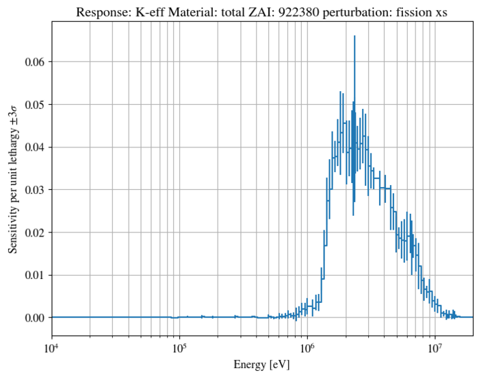
    "keff", mat="total", zai=922380, pert="fission xs",
)

# Format the plot to look like the MATLAB / OCTAVE example
# No y axis limits

pyplot.xlim(1E4, s.energies[-1]*1E6)

# Turn on minor grids for the x-axis to show the log scale better
pyplot.grid("x", which="both")
pyplot.grid("y")

# Add a title to the top of the figure
pyplot.title("Response: K-eff Material: total ZAI: 922380 perturbation: fission xs")

# Show the figure
pyplot.show()
Detailed python processing script:
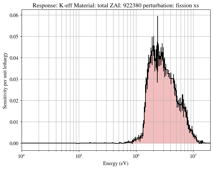
This script seeks to fully replicate the figures provided in the Wiki made using the MATLAB / OCTAVE programs
from matplotlib import pyplot
import serpentTools

s = serpentTools.read("flattop_sens.m")

# Extract the response of interest from the sensitivities dictionary

ks = s.sensitivities["keff"]

# Obtain the expected value and uncertainty by indexing into the multi-dimensional
# response. The matrix is structured [materials, isotopes, perturbations, energies, 2]
# where the last dimension stores value and uncertainty
# We can use the materials, zais, and perts dictionaries to obtain the correct index
# in each dimension for the quantity of interest

kslice = ks[
    s.materials["total"],  # index for sensitivity due to all materials
    s.zais[922380],  # index for sensitivity due to U238
    s.perts["fission xs"],  # index for sensitivity due to fission xs
]

# Normalize per unit lethargy
# Python arrays are zero-indexed, so the expected value is in the 0 index
value = kslice[:, 0] / s.lethargyWidths

# Compute 2-sigma uncertainty
unc = kslice[:, 1] * 2 * value

# Draw errorbars
# The energy vector has one additional entry, so we will instead drop the first item
# by slicing from the second position forward
pyplot.errorbar(
    s.energies[1:] * 1E6,  # convert to MeV
    value,  # expected value
    yerr=unc,   # uncertainty
    drawstyle="steps-mid",   # step-plot
    c="k",  # draw using a black line
)

# Shade the region under the curve red
# Use a mild transparency
pyplot.fill_between(s.energies[1:]*1E6, value, color="tab:red", alpha=0.3, step="mid")

# Format the plot
pyplot.xscale("log")
pyplot.xlim(1E4, s.energies[-1]*1E6)
# Major and minor grids for the log-scaled x axis
pyplot.grid("x", which="both")
pyplot.grid("y")
pyplot.xlabel("Energy (eV)")
pyplot.ylabel("Sensitivity per unit lethargy")
pyplot.title("Response: K-eff Material: total ZAI: 922380 perturbation: fission xs")

pyplot.show()
Results
Runtime of the input on a computer cluster node with a Intel Xeon E5-2690 v2 processor (10 physical cores, 20 logical cores) using 20 OpenMP threads took approximately 4 hours 50 minutes and used (allocated) 6117 MB of RAM. The run produced an 133 KB [input]_sens.m file.
Executing the processing and plotting script produced the following output using OCTAVE 4.0.0
Output from the processing script:
Results from Serpent sensitivity calculation using:

1 perturbed materials:
total

5 perturbed nuclides (ZAIs):
0
922350
922380
942390
942400

7 different perturbations:
total xs
ela scatt xs
sab scatt xs
inl scatt xs
capture xs
fission xs
nxn xs

Energy grid with 175 bins.

********************

Sensitivity results:

Material             ZAI     Perturbation         :  sensitivity | 2 sigma confidence interval
total                total   total xs             :  +0.90527000 | [ +0.90411125,  +0.90642875]
total                total   ela scatt xs         :  +0.16188300 | [ +0.16084695,  +0.16291905]
total                total   inl scatt xs         :  +0.07863120 | [ +0.07815941,  +0.07910299]
total                total   capture xs           :  -0.05447680 | [ -0.05459665,  -0.05435695]
total                total   fission xs           :  +0.71923200 | [ +0.71897308,  +0.71949092]
total                total   nxn xs               :  +0.00125871 | [ +0.00122598,  +0.00129144]

total                922350  total xs             :  +0.00818980 | [ +0.00809971,  +0.00827989]
total                922350  ela scatt xs         :  +0.00081898 | [ +0.00074855,  +0.00088941]
total                922350  inl scatt xs         :  +0.00038832 | [ +0.00035803,  +0.00041861]
total                922350  capture xs           :  -0.00054016 | [ -0.00054913,  -0.00053120]
total                922350  fission xs           :  +0.00752267 | [ +0.00747753,  +0.00756781]
total                922350  nxn xs               :  +0.00000661 | [ +0.00000463,  +0.00000859]

total                922380  total xs             :  +0.21901900 | [ +0.21805532,  +0.21998268]
total                922380  ela scatt xs         :  +0.13649800 | [ +0.13562441,  +0.13737159]
total                922380  inl scatt xs         :  +0.06499990 | [ +0.06459690,  +0.06540290]
total                922380  capture xs           :  -0.03974930 | [ -0.03986060,  -0.03963800]
total                922380  fission xs           :  +0.05727050 | [ +0.05714450,  +0.05739650]
total                922380  nxn xs               :  +0.00096484 | [ +0.00093783,  +0.00099186]

total                942390  total xs             :  +0.65488800 | [ +0.65424621,  +0.65552979]
total                942390  ela scatt xs         :  +0.02212830 | [ +0.02159722,  +0.02265938]
total                942390  inl scatt xs         :  +0.01241460 | [ +0.01216631,  +0.01266289]
total                942390  capture xs           :  -0.01294550 | [ -0.01299469,  -0.01289631]
total                942390  fission xs           :  +0.63329000 | [ +0.63301135,  +0.63356865]
total                942390  nxn xs               :  +0.00027191 | [ +0.00025614,  +0.00028768]

total                942400  total xs             :  +0.02006720 | [ +0.01991469,  +0.02021971]
total                942400  ela scatt xs         :  +0.00129135 | [ +0.00117513,  +0.00140757]
total                942400  inl scatt xs         :  +0.00063176 | [ +0.00056606,  +0.00069746]
total                942400  capture xs           :  -0.00102246 | [ -0.00103534,  -0.00100958]
total                942400  fission xs           :  +0.01916650 | [ +0.01909367,  +0.01923933]
total                942400  nxn xs               :  +0.00000945 | [ +0.00000567,  +0.00001323]
These results were obtained using ENDF/B-VII.1 based cross section libraries.
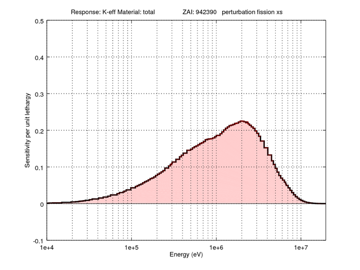
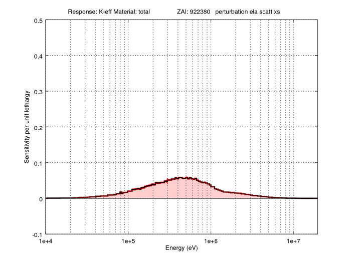
A number of produced figures are also shown here for ease of comparison:


