Difference between revisions of "Tutorial"
(→Part 5 input) |
(→Building the Serpent model for the reactor) |
||
| Line 4,229: | Line 4,229: | ||
<div class="toccolours mw-collapsible mw-expanded" style="width:60em;"> | <div class="toccolours mw-collapsible mw-expanded" style="width:60em;"> | ||
| − | '''Input for 3D research reactor geometry''' | + | '''Input for 3D research reactor geometry. Save to '''<tt>reactor</tt> |
<div class="mw-collapsible-content"> | <div class="mw-collapsible-content"> | ||
| − | + | <span style="color: Green;">% --- Research reactor input for Serpent tutorial | |
| + | |||
| + | % --- Link the materials file to this input</span> | ||
| + | |||
| + | <span style="color: Red;">include</span> "materials" | ||
| + | |||
| + | <span style="color: Green;">%%%%%%%%%%%%%%%%%%%%%%%%%%%%%%%%%%%%%%%%%%%%%%% | ||
| + | % We'll start from an infinite water geometry % | ||
| + | %%%%%%%%%%%%%%%%%%%%%%%%%%%%%%%%%%%%%%%%%%%%%%% | ||
| + | |||
| + | % --- Infinite surface as a boundary</span> | ||
| + | |||
| + | <span style="color: Red;">surf</span> <span style="color: Blue;">sINF</span> inf | ||
| + | |||
| + | <span style="color: Green;">% --- Cell cIN contains water</span> | ||
| + | |||
| + | <span style="color: Red;">cell</span> <span style="color: Blue;">cIN</span> 0 <span style="color: Purple;">water</span> -sINF | ||
| + | |||
| + | <span style="color: Green;">% --- Cell cOUT is defined as an outside cell</span> | ||
| + | |||
| + | <span style="color: Red;">cell</span> <span style="color: Blue;">cOUT</span> 0 outside sINF | ||
| + | |||
| + | <span style="color: Green;">/****************** | ||
| + | * Run parameters * | ||
| + | ******************/ | ||
| + | |||
| + | % --- Neutron population: 10000 neutrons per cycle, 100 active / 50 inactive cycles</span> | ||
| + | |||
| + | <span style="color: Red;">set pop</span> 10000 100 50 | ||
| + | |||
| + | <span style="color: Green;">% --- Geometry plots</span> | ||
| + | |||
| + | <span style="color: Green;">% --- XY-plot</span> | ||
| + | |||
| + | <span style="color: Red;">plot</span> 3 200 200 | ||
| + | |||
| + | <span style="color: Green;">% --- XZ-plot</span> | ||
| + | |||
| + | <span style="color: Red;">plot</span> 2 200 200 | ||
</div> | </div> | ||
</div> | </div> | ||
Revision as of 15:43, 14 September 2017
This page is the beginning of a hands-on tutorial in Serpent that will walk you through the creation of simple pin-cell and assembly geometry models and the use of those models for some reactor physics simulations.
Contents
- 1 Prerequisite
- 2 Basics of Serpent input
- 3 Part 1: Infinite homogeneous system
- 4 Part 2: A 2D pin-cell (infinite lattice)
- 5 Part 3: A 2D assembly model (infinite lattice)
- 6 Part 4: Assembly burnup calculation
- 7 Part 5: A 3D research reactor model
- 8 References
Prerequisite
Compiled version of Serpent 2.
This tutorial assumes that you can run Serpent 2 simply by typing sss2 in your terminal, i.e. you either have the executable in your PATH or have created an alias for the executable. If this is not the case, you'll need to replace the sss2 run-commands with the full path to your executable.
Cross section libraries.
This tutorial assumes that you have defined a default cross section directory file for Serpent using the SERPENT_ACELIB environment variable (see the notes of set acelib). If this is not the case, you'll need to give the path to a cross section directory file in the input using set acelib.
Basics of Serpent input
Explain different (typical) parts such as:
- Material definitions
- Geometry definitions
- Run parameters/options
Part 1: Infinite homogeneous system
Part 1 overview
The first model in this tutorial is the simplest geometry model one can imagine: an infinite homogeneous system consisting of a single material. Here the infinite material is 4.0 wt-% enriched uranium with a density of 10.1 g/cm3.
We will use the infinite homogeneous system example for three tasks:
- Finding the critical enrichment of an infinite uranium system.
- Tallying the neutron energy spectrum in the critical infinite uranium system.
- Testing the effect of added neutron moderation on the multiplication factor and energy spectrum of the system.
Part 1 input
The input of the model is shown below and consists of only five definitions:
- Defining the single material, which is called fuel in this example.
- Defining the geometry by
- Defining an "infinite" surface, i.e. a surface enclosing all of space. The surface name is s1 in this example.
- Defining two geometry cells: One containing the material fuel and the other being defined as an outside cell.
- Setting up any other run parameters, here simply setting the neutron population that is to be simulated.
Copy and paste the input below to a file named infinite on your computer.
Colors in the input correspond to:
- Comments: These are ignored by Serpent.
- Control words: A constantly updating list of control words can be found in the Input syntax manual. Everything between two control words that is not a comment is treated as a parameter to the first control word.
- Name definitions: Name definitions for the various Serpent objects can contain characters and numbers and are used for referencing certain objects in other definitions.
- Name references: References to named objects defined in the input. Name references can be made even if the name definition has not been made yet as long as the name will be defined later in the input.
Running the input for the infinite system
Simply run the input from terminal, by being in the same directory as the input-file and executing
sss2 infinite
If you compiled Serpent with OpenMP libraries for parallel computing, you can run the input with multiple OpenMP threads to use more than one processor:
sss2 -omp N infinite
where N is the number of OpenMP threads you want to use and can be set to, e.g. the number of available processor cores.
An example of the expected output is given below, although you should note that the statistical nature of the Monte Carlo methods means that you will not get exactly same values for the k-effective:
Expected output for the infinite system
_ .-=-. .-=-. .-==-.
{ } __ .' O o '. .' O o '. / -<' )--<
{ } .' O'. / o .-. O \ / o .-. O \ / .---`
{ } / .-. o\ /O / \ o\ /O / \ o\ /O /
\ `-` / \ O`-'o / \ O`-'o / \ O`-`o /
`-.-` '.____.' `._____.' `.____.'
Serpent 2 beta
A Continuous-energy Monte Carlo Reactor Physics Burnup Calculation Code
- Version 2.1.29 (June 12, 2017) -- Contact: serpent@vtt.fi
- Reference: J. Leppanen, et al. "The Serpent Monte Carlo code: Status,
development and applications in 2013." Ann. Nucl. Energy,
82 (2015) 142-150.
- Compiled Jun 19 2017 10:21:15
- MPI Parallel calculation mode not available
- OpenMP Parallel calculation mode available
- Geometry and mesh plotting available
- Default data path set to: "/home/vvvillehe/XSdata/"
Begin calculation on Mon Sep 11 12:51:14 2017
Reading input file "infinite"...
Checking duplicate input definitions...
OK.
Creating geometry...
OK.
Counting geometry zones...
Processing cells...
OK.
Linking materials to geometry...
OK.
Counting cells...
OK.
Processing data for group constant generation:
- 70 energy groups in micro-group structure
- 2 energy groups in macro-group structure
- B1 fundamental mode calculation is not run
- Group constants generated in 1 universes
- Discontinuity factors are not calculated
- Pin-power distributions are not calculated
- Albedos are not calculated
- Poison cross sections are not calculated
Reading ACE directory files...
OK.
Adding nuclides in material fuel...
Nuclide 92235.03c -- uranium 235 at 300K (U-235)
Nuclide 92238.03c -- uranium 238 at 300K (U-238)
Checking data and printing output...
OK.
***** Mon Sep 11 12:51:15 2017 (seed = 1505123474)
Warning message from function ProcessNuclides:
Minimum photon cross section energy 1.000000E+37 MeV is
above the energy grid minimum 1.000000E-03 MeV.
The energy grid minimum is set to 1.000000E+37 MeV.
Possible changes in energy cutoff cards (warned if any).
***** Mon Sep 11 12:51:15 2017 (seed = 1505123474)
Warning message from function ProcessNuclides:
Photon energy cutoff 1.000000E-03 MeV is changed to 1.000000E+37.
Generating unionize energy grids...
Adding points:
92235.03c -- Points added in neutron grid: 30884
92238.03c -- Points added in neutron grid: 64918
Generating unionized energy grid:
- Unionization performed without grid thinning
between 1.00E-11 and 20.0 MeV.
- Final neutron grid size: 95836 points.
- 2.12 Mb of memory allocated for grid data
OK.
Processing cross sections and ENDF reaction laws...
Nuclide 92235.03c -- uranium 235 at 300K (U-235)
Nuclide 92238.03c -- uranium 238 at 300K (U-238)
SUMMARY -- 2 nuclides included in calculation:
- 2 transport nuclides
- Neutron energy cut-offs at 1.00E-11 and 20.0 MeV
- 88 transport reactions
- 2 special reactions
- 18.07 Mb of memory allocated for data
Normalizing compositions and processing mixtures...
OK.
Allocating memory for macroscopic cross section data...
OK.
Allocating memory for particle structures...
OK.
Calculating maximum densities...
OK.
Performing density cut-off...
OK.
Sorting material-wise reaction lists:
0% complete
100% complete
Calculating macroscopic cross sections:
0% complete
100% complete
Calculating DT neutron majorant cross section:
0% complete
100% complete
Clearing results and statistics...
OK.
Sampling initial source...
OK.
Inactive cycle 1 / 20: k-eff = 1.00000
Inactive cycle 2 / 20: k-eff = 0.83420
Inactive cycle 3 / 20: k-eff = 0.79549
Inactive cycle 4 / 20: k-eff = 0.87011
Inactive cycle 5 / 20: k-eff = 0.81582
Inactive cycle 6 / 20: k-eff = 0.83654
Inactive cycle 7 / 20: k-eff = 0.81429
Inactive cycle 8 / 20: k-eff = 0.88334
Inactive cycle 9 / 20: k-eff = 0.84641
Inactive cycle 10 / 20: k-eff = 0.88078
Inactive cycle 11 / 20: k-eff = 0.82141
Inactive cycle 12 / 20: k-eff = 0.83916
Inactive cycle 13 / 20: k-eff = 0.85225
Inactive cycle 14 / 20: k-eff = 0.84424
Inactive cycle 15 / 20: k-eff = 0.82836
Inactive cycle 16 / 20: k-eff = 0.80235
Inactive cycle 17 / 20: k-eff = 0.84424
Inactive cycle 18 / 20: k-eff = 0.85251
Inactive cycle 19 / 20: k-eff = 0.81653
Inactive cycle 20 / 20: k-eff = 0.83237
----- Begin active cycles -----
------------------------------------------------------------
Serpent 2.1.29 -- Static criticality source simulation
Input file: "infinite"
Active cycle 1 / 100 Source neutrons : 5177
Running time : 0:00:09
Estimated running time : -:--:--
Estimated running time left : -:--:--
Estimated relative CPU usage : 100.0%
k-eff (analog) = 0.86184 +/- 0.00000 [0.86184 0.86184]
k-eff (implicit) = 0.84234 +/- 0.00000 [0.84234 0.84234]
(O4) (OMP=1)
------------------------------------------------------------
------------------------------------------------------------
Serpent 2.1.29 -- Static criticality source simulation
Input file: "infinite"
Active cycle 2 / 100 Source neutrons : 4873
Running time : 0:00:09
Estimated running time : -:--:--
Estimated running time left : -:--:--
Estimated relative CPU usage : 100.1%
k-eff (analog) = 0.85090 +/- 0.01095 [0.82944 0.87235]
k-eff (implicit) = 0.83921 +/- 0.00313 [0.83308 0.84535]
(O4) (OMP=1)
------------------------------------------------------------
------------------------------------------------------------
Serpent 2.1.29 -- Static criticality source simulation
Input file: "infinite"
Active cycle 3 / 100 Source neutrons : 4979
Running time : 0:00:10
Estimated running time : -:--:--
Estimated running time left : -:--:--
Estimated relative CPU usage : 99.9%
k-eff (analog) = 0.84607 +/- 0.00795 [0.83049 0.86165]
k-eff (implicit) = 0.83824 +/- 0.00205 [0.83421 0.84226]
(O4) (OMP=1)
------------------------------------------------------------
------------------------------------------------------------
Serpent 2.1.29 -- Static criticality source simulation
Input file: "infinite"
Active cycle 4 / 100 Source neutrons : 4980
Running time : 0:00:10
Estimated running time : -:--:--
Estimated running time left : -:--:--
Estimated relative CPU usage : 100.0%
k-eff (analog) = 0.84282 +/- 0.00649 [0.83010 0.85555]
k-eff (implicit) = 0.83595 +/- 0.00271 [0.83063 0.84127]
(O4) (OMP=1)
------------------------------------------------------------
------------------------------------------------------------
Serpent 2.1.29 -- Static criticality source simulation
Input file: "infinite"
Active cycle 5 / 100 Source neutrons : 5072
Running time : 0:00:11
Estimated running time : 0:00:57
Estimated running time left : 0:00:46
Estimated relative CPU usage : 99.9%
k-eff (analog) = 0.84327 +/- 0.00505 [0.83338 0.85317]
k-eff (implicit) = 0.83419 +/- 0.00274 [0.82882 0.83956]
(O4) (OMP=1)
------------------------------------------------------------
------------------------------------------------------------
Serpent 2.1.29 -- Static criticality source simulation
Input file: "infinite"
Active cycle 6 / 100 Source neutrons : 4895
Running time : 0:00:11
Estimated running time : 0:00:57
Estimated running time left : 0:00:45
Estimated relative CPU usage : 100.0%
k-eff (analog) = 0.84061 +/- 0.00491 [0.83100 0.85023]
k-eff (implicit) = 0.83488 +/- 0.00234 [0.83029 0.83946]
(O4) (OMP=1)
------------------------------------------------------------
------------------------------------------------------------
Serpent 2.1.29 -- Static criticality source simulation
Input file: "infinite"
Active cycle 7 / 100 Source neutrons : 5060
Running time : 0:00:12
Estimated running time : 0:00:57
Estimated running time left : 0:00:45
Estimated relative CPU usage : 99.9%
k-eff (analog) = 0.84013 +/- 0.00417 [0.83195 0.84831]
k-eff (implicit) = 0.83563 +/- 0.00212 [0.83149 0.83978]
(O4) (OMP=1)
------------------------------------------------------------
------------------------------------------------------------
Serpent 2.1.29 -- Static criticality source simulation
Input file: "infinite"
Active cycle 8 / 100 Source neutrons : 5034
Running time : 0:00:12
Estimated running time : 0:00:57
Estimated running time left : 0:00:44
Estimated relative CPU usage : 100.1%
k-eff (analog) = 0.84049 +/- 0.00363 [0.83337 0.84760]
k-eff (implicit) = 0.83605 +/- 0.00188 [0.83237 0.83974]
(O4) (OMP=1)
------------------------------------------------------------
------------------------------------------------------------
Serpent 2.1.29 -- Static criticality source simulation
Input file: "infinite"
Active cycle 9 / 100 Source neutrons : 5141
Running time : 0:00:12
Estimated running time : 0:00:56
Estimated running time left : 0:00:43
Estimated relative CPU usage : 100.0%
k-eff (analog) = 0.84340 +/- 0.00433 [0.83491 0.85189]
k-eff (implicit) = 0.83678 +/- 0.00181 [0.83323 0.84032]
(O4) (OMP=1)
------------------------------------------------------------
------------------------------------------------------------
Serpent 2.1.29 -- Static criticality source simulation
Input file: "infinite"
Active cycle 10 / 100 Source neutrons : 4689
Running time : 0:00:13
Estimated running time : 0:00:56
Estimated running time left : 0:00:43
Estimated relative CPU usage : 100.0%
k-eff (analog) = 0.84034 +/- 0.00494 [0.83067 0.85002]
k-eff (implicit) = 0.83686 +/- 0.00162 [0.83368 0.84003]
(O4) (OMP=1)
------------------------------------------------------------
------------------------------------------------------------
Serpent 2.1.29 -- Static criticality source simulation
Input file: "infinite"
Active cycle 11 / 100 Source neutrons : 5340
Running time : 0:00:13
Estimated running time : 0:00:56
Estimated running time left : 0:00:42
Estimated relative CPU usage : 100.0%
k-eff (analog) = 0.84286 +/- 0.00513 [0.83281 0.85291]
k-eff (implicit) = 0.83725 +/- 0.00152 [0.83428 0.84022]
(O4) (OMP=1)
------------------------------------------------------------
------------------------------------------------------------
Serpent 2.1.29 -- Static criticality source simulation
Input file: "infinite"
Active cycle 12 / 100 Source neutrons : 4906
Running time : 0:00:14
Estimated running time : 0:00:56
Estimated running time left : 0:00:42
Estimated relative CPU usage : 99.9%
k-eff (analog) = 0.84360 +/- 0.00474 [0.83432 0.85289]
k-eff (implicit) = 0.83862 +/- 0.00195 [0.83480 0.84243]
(O4) (OMP=1)
------------------------------------------------------------
------------------------------------------------------------
Serpent 2.1.29 -- Static criticality source simulation
Input file: "infinite"
Active cycle 13 / 100 Source neutrons : 5000
Running time : 0:00:14
Estimated running time : 0:00:56
Estimated running time left : 0:00:41
Estimated relative CPU usage : 100.0%
k-eff (analog) = 0.84423 +/- 0.00440 [0.83560 0.85286]
k-eff (implicit) = 0.83770 +/- 0.00201 [0.83376 0.84164]
(O4) (OMP=1)
------------------------------------------------------------
------------------------------------------------------------
Serpent 2.1.29 -- Static criticality source simulation
Input file: "infinite"
Active cycle 14 / 100 Source neutrons : 4759
Running time : 0:00:15
Estimated running time : 0:00:56
Estimated running time left : 0:00:41
Estimated relative CPU usage : 100.1%
k-eff (analog) = 0.84184 +/- 0.00473 [0.83257 0.85111]
k-eff (implicit) = 0.83771 +/- 0.00186 [0.83406 0.84135]
(O4) (OMP=1)
------------------------------------------------------------
------------------------------------------------------------
Serpent 2.1.29 -- Static criticality source simulation
Input file: "infinite"
Active cycle 15 / 100 Source neutrons : 5270
Running time : 0:00:15
Estimated running time : 0:00:56
Estimated running time left : 0:00:40
Estimated relative CPU usage : 100.0%
k-eff (analog) = 0.84268 +/- 0.00448 [0.83390 0.85147]
k-eff (implicit) = 0.83771 +/- 0.00173 [0.83432 0.84111]
(O4) (OMP=1)
------------------------------------------------------------
------------------------------------------------------------
Serpent 2.1.29 -- Static criticality source simulation
Input file: "infinite"
Active cycle 16 / 100 Source neutrons : 4903
Running time : 0:00:16
Estimated running time : 0:00:56
Estimated running time left : 0:00:40
Estimated relative CPU usage : 100.1%
k-eff (analog) = 0.84238 +/- 0.00420 [0.83414 0.85062]
k-eff (implicit) = 0.83794 +/- 0.00164 [0.83474 0.84115]
(O4) (OMP=1)
------------------------------------------------------------
------------------------------------------------------------
Serpent 2.1.29 -- Static criticality source simulation
Input file: "infinite"
Active cycle 17 / 100 Source neutrons : 5066
Running time : 0:00:16
Estimated running time : 0:00:56
Estimated running time left : 0:00:39
Estimated relative CPU usage : 100.2%
k-eff (analog) = 0.84277 +/- 0.00397 [0.83499 0.85054]
k-eff (implicit) = 0.83708 +/- 0.00176 [0.83363 0.84054]
(O4) (OMP=1)
------------------------------------------------------------
------------------------------------------------------------
Serpent 2.1.29 -- Static criticality source simulation
Input file: "infinite"
Active cycle 18 / 100 Source neutrons : 4864
Running time : 0:00:17
Estimated running time : 0:00:56
Estimated running time left : 0:00:39
Estimated relative CPU usage : 99.9%
k-eff (analog) = 0.84183 +/- 0.00386 [0.83427 0.84939]
k-eff (implicit) = 0.83702 +/- 0.00166 [0.83376 0.84028]
(O4) (OMP=1)
------------------------------------------------------------
------------------------------------------------------------
Serpent 2.1.29 -- Static criticality source simulation
Input file: "infinite"
Active cycle 19 / 100 Source neutrons : 5195
Running time : 0:00:17
Estimated running time : 0:00:56
Estimated running time left : 0:00:38
Estimated relative CPU usage : 100.0%
k-eff (analog) = 0.84269 +/- 0.00375 [0.83534 0.85003]
k-eff (implicit) = 0.83771 +/- 0.00172 [0.83435 0.84107]
(O4) (OMP=1)
------------------------------------------------------------
------------------------------------------------------------
Serpent 2.1.29 -- Static criticality source simulation
Input file: "infinite"
Active cycle 20 / 100 Source neutrons : 4758
Running time : 0:00:18
Estimated running time : 0:00:56
Estimated running time left : 0:00:38
Estimated relative CPU usage : 100.1%
k-eff (analog) = 0.84138 +/- 0.00379 [0.83396 0.84880]
k-eff (implicit) = 0.83786 +/- 0.00163 [0.83465 0.84106]
(O4) (OMP=1)
------------------------------------------------------------
------------------------------------------------------------
Serpent 2.1.29 -- Static criticality source simulation
Input file: "infinite"
Active cycle 21 / 100 Source neutrons : 5296
Running time : 0:00:18
Estimated running time : 0:00:56
Estimated running time left : 0:00:37
Estimated relative CPU usage : 99.9%
k-eff (analog) = 0.84250 +/- 0.00377 [0.83511 0.84989]
k-eff (implicit) = 0.83784 +/- 0.00155 [0.83480 0.84089]
(O4) (OMP=1)
------------------------------------------------------------
------------------------------------------------------------
Serpent 2.1.29 -- Static criticality source simulation
Input file: "infinite"
Active cycle 22 / 100 Source neutrons : 4817
Running time : 0:00:19
Estimated running time : 0:00:56
Estimated running time left : 0:00:37
Estimated relative CPU usage : 100.0%
k-eff (analog) = 0.84208 +/- 0.00362 [0.83498 0.84918]
k-eff (implicit) = 0.83827 +/- 0.00154 [0.83525 0.84130]
(O4) (OMP=1)
------------------------------------------------------------
------------------------------------------------------------
Serpent 2.1.29 -- Static criticality source simulation
Input file: "infinite"
Active cycle 23 / 100 Source neutrons : 5027
Running time : 0:00:19
Estimated running time : 0:00:56
Estimated running time left : 0:00:36
Estimated relative CPU usage : 100.0%
k-eff (analog) = 0.84189 +/- 0.00347 [0.83510 0.84868]
k-eff (implicit) = 0.83835 +/- 0.00148 [0.83545 0.84124]
(O4) (OMP=1)
------------------------------------------------------------
------------------------------------------------------------
Serpent 2.1.29 -- Static criticality source simulation
Input file: "infinite"
Active cycle 24 / 100 Source neutrons : 4986
Running time : 0:00:20
Estimated running time : 0:00:56
Estimated running time left : 0:00:36
Estimated relative CPU usage : 100.1%
k-eff (analog) = 0.84162 +/- 0.00333 [0.83509 0.84814]
k-eff (implicit) = 0.83830 +/- 0.00141 [0.83553 0.84107]
(O4) (OMP=1)
------------------------------------------------------------
------------------------------------------------------------
Serpent 2.1.29 -- Static criticality source simulation
Input file: "infinite"
Active cycle 25 / 100 Source neutrons : 5009
Running time : 0:00:20
Estimated running time : 0:00:56
Estimated running time left : 0:00:35
Estimated relative CPU usage : 99.9%
k-eff (analog) = 0.84143 +/- 0.00320 [0.83516 0.84770]
k-eff (implicit) = 0.83851 +/- 0.00137 [0.83582 0.84120]
(O4) (OMP=1)
------------------------------------------------------------
------------------------------------------------------------
Serpent 2.1.29 -- Static criticality source simulation
Input file: "infinite"
Active cycle 26 / 100 Source neutrons : 5049
Running time : 0:00:21
Estimated running time : 0:00:56
Estimated running time left : 0:00:35
Estimated relative CPU usage : 100.1%
k-eff (analog) = 0.84157 +/- 0.00308 [0.83554 0.84760]
k-eff (implicit) = 0.83871 +/- 0.00133 [0.83609 0.84132]
(O4) (OMP=1)
------------------------------------------------------------
------------------------------------------------------------
Serpent 2.1.29 -- Static criticality source simulation
Input file: "infinite"
Active cycle 27 / 100 Source neutrons : 5140
Running time : 0:00:21
Estimated running time : 0:00:56
Estimated running time left : 0:00:35
Estimated relative CPU usage : 99.9%
k-eff (analog) = 0.84258 +/- 0.00313 [0.83645 0.84871]
k-eff (implicit) = 0.83871 +/- 0.00128 [0.83620 0.84123]
(O4) (OMP=1)
------------------------------------------------------------
------------------------------------------------------------
Serpent 2.1.29 -- Static criticality source simulation
Input file: "infinite"
Active cycle 28 / 100 Source neutrons : 4907
Running time : 0:00:22
Estimated running time : 0:00:56
Estimated running time left : 0:00:34
Estimated relative CPU usage : 100.1%
k-eff (analog) = 0.84294 +/- 0.00303 [0.83699 0.84888]
k-eff (implicit) = 0.83878 +/- 0.00124 [0.83635 0.84120]
(O4) (OMP=1)
------------------------------------------------------------
------------------------------------------------------------
Serpent 2.1.29 -- Static criticality source simulation
Input file: "infinite"
Active cycle 29 / 100 Source neutrons : 4885
Running time : 0:00:22
Estimated running time : 0:00:57
Estimated running time left : 0:00:34
Estimated relative CPU usage : 99.8%
k-eff (analog) = 0.84259 +/- 0.00295 [0.83681 0.84837]
k-eff (implicit) = 0.83902 +/- 0.00122 [0.83663 0.84140]
(O4) (OMP=1)
------------------------------------------------------------
------------------------------------------------------------
Serpent 2.1.29 -- Static criticality source simulation
Input file: "infinite"
Active cycle 30 / 100 Source neutrons : 5101
Running time : 0:00:23
Estimated running time : 0:00:57
Estimated running time left : 0:00:33
Estimated relative CPU usage : 100.1%
k-eff (analog) = 0.84283 +/- 0.00286 [0.83723 0.84843]
k-eff (implicit) = 0.83909 +/- 0.00118 [0.83678 0.84140]
(O4) (OMP=1)
------------------------------------------------------------
------------------------------------------------------------
Serpent 2.1.29 -- Static criticality source simulation
Input file: "infinite"
Active cycle 31 / 100 Source neutrons : 4844
Running time : 0:00:23
Estimated running time : 0:00:56
Estimated running time left : 0:00:33
Estimated relative CPU usage : 100.0%
k-eff (analog) = 0.84220 +/- 0.00284 [0.83665 0.84776]
k-eff (implicit) = 0.83927 +/- 0.00115 [0.83700 0.84153]
(O4) (OMP=1)
------------------------------------------------------------
------------------------------------------------------------
Serpent 2.1.29 -- Static criticality source simulation
Input file: "infinite"
Active cycle 32 / 100 Source neutrons : 5069
Running time : 0:00:24
Estimated running time : 0:00:56
Estimated running time left : 0:00:32
Estimated relative CPU usage : 100.2%
k-eff (analog) = 0.84197 +/- 0.00276 [0.83657 0.84737]
k-eff (implicit) = 0.83902 +/- 0.00114 [0.83678 0.84126]
(O4) (OMP=1)
------------------------------------------------------------
------------------------------------------------------------
Serpent 2.1.29 -- Static criticality source simulation
Input file: "infinite"
Active cycle 33 / 100 Source neutrons : 5146
Running time : 0:00:24
Estimated running time : 0:00:57
Estimated running time left : 0:00:32
Estimated relative CPU usage : 99.9%
k-eff (analog) = 0.84248 +/- 0.00272 [0.83715 0.84782]
k-eff (implicit) = 0.83844 +/- 0.00125 [0.83598 0.84089]
(O4) (OMP=1)
------------------------------------------------------------
------------------------------------------------------------
Serpent 2.1.29 -- Static criticality source simulation
Input file: "infinite"
Active cycle 34 / 100 Source neutrons : 4777
Running time : 0:00:25
Estimated running time : 0:00:57
Estimated running time left : 0:00:32
Estimated relative CPU usage : 100.0%
k-eff (analog) = 0.84184 +/- 0.00272 [0.83652 0.84717]
k-eff (implicit) = 0.83807 +/- 0.00127 [0.83558 0.84056]
(O4) (OMP=1)
------------------------------------------------------------
------------------------------------------------------------
Serpent 2.1.29 -- Static criticality source simulation
Input file: "infinite"
Active cycle 35 / 100 Source neutrons : 5022
Running time : 0:00:25
Estimated running time : 0:00:57
Estimated running time left : 0:00:31
Estimated relative CPU usage : 100.0%
k-eff (analog) = 0.84134 +/- 0.00268 [0.83608 0.84660]
k-eff (implicit) = 0.83781 +/- 0.00126 [0.83534 0.84028]
(O4) (OMP=1)
------------------------------------------------------------
------------------------------------------------------------
Serpent 2.1.29 -- Static criticality source simulation
Input file: "infinite"
Active cycle 36 / 100 Source neutrons : 4947
Running time : 0:00:26
Estimated running time : 0:00:57
Estimated running time left : 0:00:31
Estimated relative CPU usage : 100.0%
k-eff (analog) = 0.84063 +/- 0.00270 [0.83533 0.84593]
k-eff (implicit) = 0.83794 +/- 0.00123 [0.83553 0.84035]
(O4) (OMP=1)
------------------------------------------------------------
------------------------------------------------------------
Serpent 2.1.29 -- Static criticality source simulation
Input file: "infinite"
Active cycle 37 / 100 Source neutrons : 5137
Running time : 0:00:26
Estimated running time : 0:00:57
Estimated running time left : 0:00:30
Estimated relative CPU usage : 100.1%
k-eff (analog) = 0.84056 +/- 0.00263 [0.83540 0.84571]
k-eff (implicit) = 0.83793 +/- 0.00120 [0.83559 0.84028]
(O4) (OMP=1)
------------------------------------------------------------
------------------------------------------------------------
Serpent 2.1.29 -- Static criticality source simulation
Input file: "infinite"
Active cycle 38 / 100 Source neutrons : 5042
Running time : 0:00:27
Estimated running time : 0:00:57
Estimated running time left : 0:00:30
Estimated relative CPU usage : 100.0%
k-eff (analog) = 0.84067 +/- 0.00256 [0.83565 0.84570]
k-eff (implicit) = 0.83794 +/- 0.00117 [0.83566 0.84023]
(O4) (OMP=1)
------------------------------------------------------------
------------------------------------------------------------
Serpent 2.1.29 -- Static criticality source simulation
Input file: "infinite"
Active cycle 39 / 100 Source neutrons : 5086
Running time : 0:00:27
Estimated running time : 0:00:57
Estimated running time left : 0:00:29
Estimated relative CPU usage : 100.0%
k-eff (analog) = 0.84116 +/- 0.00254 [0.83617 0.84614]
k-eff (implicit) = 0.83800 +/- 0.00114 [0.83577 0.84022]
(O4) (OMP=1)
------------------------------------------------------------
------------------------------------------------------------
Serpent 2.1.29 -- Static criticality source simulation
Input file: "infinite"
Active cycle 40 / 100 Source neutrons : 4784
Running time : 0:00:28
Estimated running time : 0:00:57
Estimated running time left : 0:00:29
Estimated relative CPU usage : 100.0%
k-eff (analog) = 0.84069 +/- 0.00252 [0.83574 0.84563]
k-eff (implicit) = 0.83796 +/- 0.00111 [0.83579 0.84013]
(O4) (OMP=1)
------------------------------------------------------------
------------------------------------------------------------
Serpent 2.1.29 -- Static criticality source simulation
Input file: "infinite"
Active cycle 41 / 100 Source neutrons : 5005
Running time : 0:00:28
Estimated running time : 0:00:57
Estimated running time left : 0:00:28
Estimated relative CPU usage : 100.0%
k-eff (analog) = 0.84026 +/- 0.00250 [0.83537 0.84516]
k-eff (implicit) = 0.83810 +/- 0.00109 [0.83597 0.84024]
(O4) (OMP=1)
------------------------------------------------------------
------------------------------------------------------------
Serpent 2.1.29 -- Static criticality source simulation
Input file: "infinite"
Active cycle 42 / 100 Source neutrons : 5001
Running time : 0:00:29
Estimated running time : 0:00:57
Estimated running time left : 0:00:28
Estimated relative CPU usage : 99.9%
k-eff (analog) = 0.83986 +/- 0.00247 [0.83502 0.84470]
k-eff (implicit) = 0.83831 +/- 0.00108 [0.83619 0.84044]
(O4) (OMP=1)
------------------------------------------------------------
------------------------------------------------------------
Serpent 2.1.29 -- Static criticality source simulation
Input file: "infinite"
Active cycle 43 / 100 Source neutrons : 4897
Running time : 0:00:29
Estimated running time : 0:00:57
Estimated running time left : 0:00:27
Estimated relative CPU usage : 100.1%
k-eff (analog) = 0.83908 +/- 0.00253 [0.83411 0.84405]
k-eff (implicit) = 0.83816 +/- 0.00107 [0.83606 0.84025]
(O4) (OMP=1)
------------------------------------------------------------
------------------------------------------------------------
Serpent 2.1.29 -- Static criticality source simulation
Input file: "infinite"
Active cycle 44 / 100 Source neutrons : 5279
Running time : 0:00:29
Estimated running time : 0:00:57
Estimated running time left : 0:00:27
Estimated relative CPU usage : 100.0%
k-eff (analog) = 0.83936 +/- 0.00249 [0.83448 0.84424]
k-eff (implicit) = 0.83805 +/- 0.00105 [0.83599 0.84011]
(O4) (OMP=1)
------------------------------------------------------------
------------------------------------------------------------
Serpent 2.1.29 -- Static criticality source simulation
Input file: "infinite"
Active cycle 45 / 100 Source neutrons : 4871
Running time : 0:00:30
Estimated running time : 0:00:57
Estimated running time left : 0:00:26
Estimated relative CPU usage : 99.9%
k-eff (analog) = 0.83914 +/- 0.00245 [0.83435 0.84393]
k-eff (implicit) = 0.83832 +/- 0.00106 [0.83624 0.84041]
(O4) (OMP=1)
------------------------------------------------------------
------------------------------------------------------------
Serpent 2.1.29 -- Static criticality source simulation
Input file: "infinite"
Active cycle 46 / 100 Source neutrons : 5106
Running time : 0:00:30
Estimated running time : 0:00:57
Estimated running time left : 0:00:26
Estimated relative CPU usage : 100.1%
k-eff (analog) = 0.83931 +/- 0.00240 [0.83461 0.84401]
k-eff (implicit) = 0.83830 +/- 0.00104 [0.83626 0.84034]
(O4) (OMP=1)
------------------------------------------------------------
------------------------------------------------------------
Serpent 2.1.29 -- Static criticality source simulation
Input file: "infinite"
Active cycle 47 / 100 Source neutrons : 4952
Running time : 0:00:31
Estimated running time : 0:00:57
Estimated running time left : 0:00:25
Estimated relative CPU usage : 100.0%
k-eff (analog) = 0.83930 +/- 0.00235 [0.83470 0.84390]
k-eff (implicit) = 0.83833 +/- 0.00102 [0.83634 0.84033]
(O4) (OMP=1)
------------------------------------------------------------
------------------------------------------------------------
Serpent 2.1.29 -- Static criticality source simulation
Input file: "infinite"
Active cycle 48 / 100 Source neutrons : 5081
Running time : 0:00:31
Estimated running time : 0:00:57
Estimated running time left : 0:00:25
Estimated relative CPU usage : 100.0%
k-eff (analog) = 0.83958 +/- 0.00231 [0.83504 0.84411]
k-eff (implicit) = 0.83828 +/- 0.00100 [0.83632 0.84023]
(O4) (OMP=1)
------------------------------------------------------------
------------------------------------------------------------
Serpent 2.1.29 -- Static criticality source simulation
Input file: "infinite"
Active cycle 49 / 100 Source neutrons : 4830
Running time : 0:00:32
Estimated running time : 0:00:56
Estimated running time left : 0:00:24
Estimated relative CPU usage : 99.9%
k-eff (analog) = 0.83925 +/- 0.00229 [0.83476 0.84374]
k-eff (implicit) = 0.83831 +/- 0.00098 [0.83640 0.84023]
(O4) (OMP=1)
------------------------------------------------------------
------------------------------------------------------------
Serpent 2.1.29 -- Static criticality source simulation
Input file: "infinite"
Active cycle 50 / 100 Source neutrons : 5171
Running time : 0:00:32
Estimated running time : 0:00:56
Estimated running time left : 0:00:24
Estimated relative CPU usage : 100.0%
k-eff (analog) = 0.83950 +/- 0.00226 [0.83507 0.84392]
k-eff (implicit) = 0.83848 +/- 0.00097 [0.83657 0.84038]
(O4) (OMP=1)
------------------------------------------------------------
------------------------------------------------------------
Serpent 2.1.29 -- Static criticality source simulation
Input file: "infinite"
Active cycle 51 / 100 Source neutrons : 4947
Running time : 0:00:33
Estimated running time : 0:00:56
Estimated running time left : 0:00:23
Estimated relative CPU usage : 99.9%
k-eff (analog) = 0.83956 +/- 0.00221 [0.83522 0.84390]
k-eff (implicit) = 0.83843 +/- 0.00095 [0.83656 0.84030]
(O4) (OMP=1)
------------------------------------------------------------
------------------------------------------------------------
Serpent 2.1.29 -- Static criticality source simulation
Input file: "infinite"
Active cycle 52 / 100 Source neutrons : 4832
Running time : 0:00:33
Estimated running time : 0:00:56
Estimated running time left : 0:00:23
Estimated relative CPU usage : 100.1%
k-eff (analog) = 0.83907 +/- 0.00222 [0.83472 0.84343]
k-eff (implicit) = 0.83841 +/- 0.00094 [0.83658 0.84025]
(O4) (OMP=1)
------------------------------------------------------------
------------------------------------------------------------
Serpent 2.1.29 -- Static criticality source simulation
Input file: "infinite"
Active cycle 53 / 100 Source neutrons : 5104
Running time : 0:00:34
Estimated running time : 0:00:56
Estimated running time left : 0:00:22
Estimated relative CPU usage : 99.9%
k-eff (analog) = 0.83893 +/- 0.00219 [0.83464 0.84321]
k-eff (implicit) = 0.83842 +/- 0.00092 [0.83662 0.84022]
(O4) (OMP=1)
------------------------------------------------------------
------------------------------------------------------------
Serpent 2.1.29 -- Static criticality source simulation
Input file: "infinite"
Active cycle 54 / 100 Source neutrons : 4947
Running time : 0:00:34
Estimated running time : 0:00:56
Estimated running time left : 0:00:22
Estimated relative CPU usage : 99.9%
k-eff (analog) = 0.83862 +/- 0.00217 [0.83437 0.84287]
k-eff (implicit) = 0.83824 +/- 0.00092 [0.83644 0.84004]
(O4) (OMP=1)
------------------------------------------------------------
------------------------------------------------------------
Serpent 2.1.29 -- Static criticality source simulation
Input file: "infinite"
Active cycle 55 / 100 Source neutrons : 5038
Running time : 0:00:35
Estimated running time : 0:00:56
Estimated running time left : 0:00:21
Estimated relative CPU usage : 100.0%
k-eff (analog) = 0.83844 +/- 0.00213 [0.83426 0.84263]
k-eff (implicit) = 0.83817 +/- 0.00091 [0.83640 0.83995]
(O4) (OMP=1)
------------------------------------------------------------
------------------------------------------------------------
Serpent 2.1.29 -- Static criticality source simulation
Input file: "infinite"
Active cycle 56 / 100 Source neutrons : 5084
Running time : 0:00:35
Estimated running time : 0:00:56
Estimated running time left : 0:00:21
Estimated relative CPU usage : 100.0%
k-eff (analog) = 0.83852 +/- 0.00210 [0.83440 0.84263]
k-eff (implicit) = 0.83809 +/- 0.00089 [0.83634 0.83984]
(O4) (OMP=1)
------------------------------------------------------------
------------------------------------------------------------
Serpent 2.1.29 -- Static criticality source simulation
Input file: "infinite"
Active cycle 57 / 100 Source neutrons : 4909
Running time : 0:00:36
Estimated running time : 0:00:56
Estimated running time left : 0:00:20
Estimated relative CPU usage : 100.1%
k-eff (analog) = 0.83832 +/- 0.00207 [0.83426 0.84238]
k-eff (implicit) = 0.83820 +/- 0.00088 [0.83647 0.83993]
(O4) (OMP=1)
------------------------------------------------------------
------------------------------------------------------------
Serpent 2.1.29 -- Static criticality source simulation
Input file: "infinite"
Active cycle 58 / 100 Source neutrons : 4951
Running time : 0:00:36
Estimated running time : 0:00:56
Estimated running time left : 0:00:20
Estimated relative CPU usage : 100.0%
k-eff (analog) = 0.83799 +/- 0.00206 [0.83395 0.84203]
k-eff (implicit) = 0.83813 +/- 0.00087 [0.83642 0.83984]
(O4) (OMP=1)
------------------------------------------------------------
------------------------------------------------------------
Serpent 2.1.29 -- Static criticality source simulation
Input file: "infinite"
Active cycle 59 / 100 Source neutrons : 5098
Running time : 0:00:37
Estimated running time : 0:00:56
Estimated running time left : 0:00:19
Estimated relative CPU usage : 99.9%
k-eff (analog) = 0.83794 +/- 0.00203 [0.83397 0.84191]
k-eff (implicit) = 0.83818 +/- 0.00086 [0.83650 0.83986]
(O4) (OMP=1)
------------------------------------------------------------
------------------------------------------------------------
Serpent 2.1.29 -- Static criticality source simulation
Input file: "infinite"
Active cycle 60 / 100 Source neutrons : 4836
Running time : 0:00:37
Estimated running time : 0:00:56
Estimated running time left : 0:00:19
Estimated relative CPU usage : 100.1%
k-eff (analog) = 0.83744 +/- 0.00205 [0.83341 0.84147]
k-eff (implicit) = 0.83792 +/- 0.00088 [0.83619 0.83965]
(O4) (OMP=1)
------------------------------------------------------------
------------------------------------------------------------
Serpent 2.1.29 -- Static criticality source simulation
Input file: "infinite"
Active cycle 61 / 100 Source neutrons : 5255
Running time : 0:00:38
Estimated running time : 0:00:56
Estimated running time left : 0:00:18
Estimated relative CPU usage : 99.9%
k-eff (analog) = 0.83763 +/- 0.00203 [0.83365 0.84161]
k-eff (implicit) = 0.83793 +/- 0.00087 [0.83623 0.83963]
(O4) (OMP=1)
------------------------------------------------------------
------------------------------------------------------------
Serpent 2.1.29 -- Static criticality source simulation
Input file: "infinite"
Active cycle 62 / 100 Source neutrons : 4846
Running time : 0:00:38
Estimated running time : 0:00:56
Estimated running time left : 0:00:18
Estimated relative CPU usage : 100.0%
k-eff (analog) = 0.83739 +/- 0.00201 [0.83345 0.84133]
k-eff (implicit) = 0.83783 +/- 0.00086 [0.83614 0.83951]
(O4) (OMP=1)
------------------------------------------------------------
------------------------------------------------------------
Serpent 2.1.29 -- Static criticality source simulation
Input file: "infinite"
Active cycle 63 / 100 Source neutrons : 5153
Running time : 0:00:39
Estimated running time : 0:00:56
Estimated running time left : 0:00:17
Estimated relative CPU usage : 100.1%
k-eff (analog) = 0.83756 +/- 0.00199 [0.83367 0.84145]
k-eff (implicit) = 0.83787 +/- 0.00085 [0.83621 0.83953]
(O4) (OMP=1)
------------------------------------------------------------
------------------------------------------------------------
Serpent 2.1.29 -- Static criticality source simulation
Input file: "infinite"
Active cycle 64 / 100 Source neutrons : 4940
Running time : 0:00:39
Estimated running time : 0:00:56
Estimated running time left : 0:00:17
Estimated relative CPU usage : 100.0%
k-eff (analog) = 0.83757 +/- 0.00195 [0.83374 0.84140]
k-eff (implicit) = 0.83778 +/- 0.00084 [0.83614 0.83942]
(O4) (OMP=1)
------------------------------------------------------------
------------------------------------------------------------
Serpent 2.1.29 -- Static criticality source simulation
Input file: "infinite"
Active cycle 65 / 100 Source neutrons : 5114
Running time : 0:00:40
Estimated running time : 0:00:56
Estimated running time left : 0:00:16
Estimated relative CPU usage : 100.0%
k-eff (analog) = 0.83787 +/- 0.00195 [0.83405 0.84168]
k-eff (implicit) = 0.83770 +/- 0.00083 [0.83607 0.83932]
(O4) (OMP=1)
------------------------------------------------------------
------------------------------------------------------------
Serpent 2.1.29 -- Static criticality source simulation
Input file: "infinite"
Active cycle 66 / 100 Source neutrons : 4874
Running time : 0:00:40
Estimated running time : 0:00:56
Estimated running time left : 0:00:16
Estimated relative CPU usage : 100.0%
k-eff (analog) = 0.83783 +/- 0.00192 [0.83407 0.84159]
k-eff (implicit) = 0.83762 +/- 0.00082 [0.83601 0.83923]
(O4) (OMP=1)
------------------------------------------------------------
------------------------------------------------------------
Serpent 2.1.29 -- Static criticality source simulation
Input file: "infinite"
Active cycle 67 / 100 Source neutrons : 5093
Running time : 0:00:41
Estimated running time : 0:00:57
Estimated running time left : 0:00:15
Estimated relative CPU usage : 99.9%
k-eff (analog) = 0.83802 +/- 0.00190 [0.83430 0.84175]
k-eff (implicit) = 0.83742 +/- 0.00083 [0.83579 0.83906]
(O4) (OMP=1)
------------------------------------------------------------
------------------------------------------------------------
Serpent 2.1.29 -- Static criticality source simulation
Input file: "infinite"
Active cycle 68 / 100 Source neutrons : 4720
Running time : 0:00:41
Estimated running time : 0:00:57
Estimated running time left : 0:00:15
Estimated relative CPU usage : 100.0%
k-eff (analog) = 0.83751 +/- 0.00194 [0.83371 0.84131]
k-eff (implicit) = 0.83748 +/- 0.00082 [0.83587 0.83909]
(O4) (OMP=1)
------------------------------------------------------------
------------------------------------------------------------
Serpent 2.1.29 -- Static criticality source simulation
Input file: "infinite"
Active cycle 69 / 100 Source neutrons : 5186
Running time : 0:00:42
Estimated running time : 0:00:57
Estimated running time left : 0:00:15
Estimated relative CPU usage : 99.9%
k-eff (analog) = 0.83745 +/- 0.00191 [0.83370 0.84120]
k-eff (implicit) = 0.83738 +/- 0.00082 [0.83578 0.83898]
(O4) (OMP=1)
------------------------------------------------------------
------------------------------------------------------------
Serpent 2.1.29 -- Static criticality source simulation
Input file: "infinite"
Active cycle 70 / 100 Source neutrons : 4945
Running time : 0:00:42
Estimated running time : 0:00:57
Estimated running time left : 0:00:14
Estimated relative CPU usage : 100.1%
k-eff (analog) = 0.83726 +/- 0.00189 [0.83355 0.84097]
k-eff (implicit) = 0.83733 +/- 0.00081 [0.83575 0.83891]
(O4) (OMP=1)
------------------------------------------------------------
------------------------------------------------------------
Serpent 2.1.29 -- Static criticality source simulation
Input file: "infinite"
Active cycle 71 / 100 Source neutrons : 5134
Running time : 0:00:43
Estimated running time : 0:00:57
Estimated running time left : 0:00:14
Estimated relative CPU usage : 99.9%
k-eff (analog) = 0.83738 +/- 0.00187 [0.83372 0.84105]
k-eff (implicit) = 0.83724 +/- 0.00080 [0.83567 0.83880]
(O4) (OMP=1)
------------------------------------------------------------
------------------------------------------------------------
Serpent 2.1.29 -- Static criticality source simulation
Input file: "infinite"
Active cycle 72 / 100 Source neutrons : 4762
Running time : 0:00:43
Estimated running time : 0:00:57
Estimated running time left : 0:00:13
Estimated relative CPU usage : 100.0%
k-eff (analog) = 0.83694 +/- 0.00190 [0.83323 0.84066]
k-eff (implicit) = 0.83734 +/- 0.00080 [0.83578 0.83890]
(O4) (OMP=1)
------------------------------------------------------------
------------------------------------------------------------
Serpent 2.1.29 -- Static criticality source simulation
Input file: "infinite"
Active cycle 73 / 100 Source neutrons : 5208
Running time : 0:00:44
Estimated running time : 0:00:57
Estimated running time left : 0:00:13
Estimated relative CPU usage : 100.0%
k-eff (analog) = 0.83698 +/- 0.00187 [0.83331 0.84064]
k-eff (implicit) = 0.83739 +/- 0.00079 [0.83585 0.83893]
(O4) (OMP=1)
------------------------------------------------------------
------------------------------------------------------------
Serpent 2.1.29 -- Static criticality source simulation
Input file: "infinite"
Active cycle 74 / 100 Source neutrons : 5074
Running time : 0:00:44
Estimated running time : 0:00:57
Estimated running time left : 0:00:12
Estimated relative CPU usage : 100.1%
k-eff (analog) = 0.83718 +/- 0.00186 [0.83354 0.84081]
k-eff (implicit) = 0.83727 +/- 0.00078 [0.83573 0.83880]
(O4) (OMP=1)
------------------------------------------------------------
------------------------------------------------------------
Serpent 2.1.29 -- Static criticality source simulation
Input file: "infinite"
Active cycle 75 / 100 Source neutrons : 4814
Running time : 0:00:45
Estimated running time : 0:00:57
Estimated running time left : 0:00:12
Estimated relative CPU usage : 100.1%
k-eff (analog) = 0.83695 +/- 0.00185 [0.83333 0.84057]
k-eff (implicit) = 0.83721 +/- 0.00078 [0.83569 0.83873]
(O4) (OMP=1)
------------------------------------------------------------
------------------------------------------------------------
Serpent 2.1.29 -- Static criticality source simulation
Input file: "infinite"
Active cycle 76 / 100 Source neutrons : 5117
Running time : 0:00:45
Estimated running time : 0:00:57
Estimated running time left : 0:00:11
Estimated relative CPU usage : 99.9%
k-eff (analog) = 0.83698 +/- 0.00182 [0.83341 0.84055]
k-eff (implicit) = 0.83719 +/- 0.00077 [0.83568 0.83869]
(O4) (OMP=1)
------------------------------------------------------------
------------------------------------------------------------
Serpent 2.1.29 -- Static criticality source simulation
Input file: "infinite"
Active cycle 77 / 100 Source neutrons : 4981
Running time : 0:00:46
Estimated running time : 0:00:57
Estimated running time left : 0:00:11
Estimated relative CPU usage : 100.0%
k-eff (analog) = 0.83697 +/- 0.00180 [0.83345 0.84049]
k-eff (implicit) = 0.83715 +/- 0.00076 [0.83566 0.83863]
(O4) (OMP=1)
------------------------------------------------------------
------------------------------------------------------------
Serpent 2.1.29 -- Static criticality source simulation
Input file: "infinite"
Active cycle 78 / 100 Source neutrons : 4892
Running time : 0:00:46
Estimated running time : 0:00:57
Estimated running time left : 0:00:10
Estimated relative CPU usage : 100.0%
k-eff (analog) = 0.83672 +/- 0.00179 [0.83322 0.84023]
k-eff (implicit) = 0.83720 +/- 0.00075 [0.83573 0.83867]
(O4) (OMP=1)
------------------------------------------------------------
------------------------------------------------------------
Serpent 2.1.29 -- Static criticality source simulation
Input file: "infinite"
Active cycle 79 / 100 Source neutrons : 5267
Running time : 0:00:47
Estimated running time : 0:00:57
Estimated running time left : 0:00:10
Estimated relative CPU usage : 100.0%
k-eff (analog) = 0.83704 +/- 0.00180 [0.83352 0.84056]
k-eff (implicit) = 0.83719 +/- 0.00074 [0.83574 0.83864]
(O4) (OMP=1)
------------------------------------------------------------
------------------------------------------------------------
Serpent 2.1.29 -- Static criticality source simulation
Input file: "infinite"
Active cycle 80 / 100 Source neutrons : 4790
Running time : 0:00:47
Estimated running time : 0:00:57
Estimated running time left : 0:00:09
Estimated relative CPU usage : 99.9%
k-eff (analog) = 0.83690 +/- 0.00178 [0.83341 0.84038]
k-eff (implicit) = 0.83720 +/- 0.00073 [0.83577 0.83863]
(O4) (OMP=1)
------------------------------------------------------------
------------------------------------------------------------
Serpent 2.1.29 -- Static criticality source simulation
Input file: "infinite"
Active cycle 81 / 100 Source neutrons : 4876
Running time : 0:00:48
Estimated running time : 0:00:57
Estimated running time left : 0:00:09
Estimated relative CPU usage : 100.1%
k-eff (analog) = 0.83650 +/- 0.00180 [0.83297 0.84003]
k-eff (implicit) = 0.83721 +/- 0.00072 [0.83580 0.83863]
(O4) (OMP=1)
------------------------------------------------------------
------------------------------------------------------------
Serpent 2.1.29 -- Static criticality source simulation
Input file: "infinite"
Active cycle 82 / 100 Source neutrons : 5004
Running time : 0:00:48
Estimated running time : 0:00:57
Estimated running time left : 0:00:08
Estimated relative CPU usage : 99.9%
k-eff (analog) = 0.83613 +/- 0.00182 [0.83256 0.83969]
k-eff (implicit) = 0.83721 +/- 0.00071 [0.83581 0.83860]
(O4) (OMP=1)
------------------------------------------------------------
------------------------------------------------------------
Serpent 2.1.29 -- Static criticality source simulation
Input file: "infinite"
Active cycle 83 / 100 Source neutrons : 5153
Running time : 0:00:49
Estimated running time : 0:00:57
Estimated running time left : 0:00:08
Estimated relative CPU usage : 99.9%
k-eff (analog) = 0.83606 +/- 0.00180 [0.83254 0.83958]
k-eff (implicit) = 0.83719 +/- 0.00070 [0.83581 0.83857]
(O4) (OMP=1)
------------------------------------------------------------
------------------------------------------------------------
Serpent 2.1.29 -- Static criticality source simulation
Input file: "infinite"
Active cycle 84 / 100 Source neutrons : 5087
Running time : 0:00:49
Estimated running time : 0:00:57
Estimated running time left : 0:00:07
Estimated relative CPU usage : 100.0%
k-eff (analog) = 0.83616 +/- 0.00178 [0.83268 0.83965]
k-eff (implicit) = 0.83711 +/- 0.00070 [0.83574 0.83849]
(O4) (OMP=1)
------------------------------------------------------------
------------------------------------------------------------
Serpent 2.1.29 -- Static criticality source simulation
Input file: "infinite"
Active cycle 85 / 100 Source neutrons : 4976
Running time : 0:00:50
Estimated running time : 0:00:57
Estimated running time left : 0:00:07
Estimated relative CPU usage : 100.0%
k-eff (analog) = 0.83621 +/- 0.00176 [0.83277 0.83966]
k-eff (implicit) = 0.83705 +/- 0.00069 [0.83568 0.83841]
(O4) (OMP=1)
------------------------------------------------------------
------------------------------------------------------------
Serpent 2.1.29 -- Static criticality source simulation
Input file: "infinite"
Active cycle 86 / 100 Source neutrons : 5022
Running time : 0:00:50
Estimated running time : 0:00:57
Estimated running time left : 0:00:06
Estimated relative CPU usage : 100.0%
k-eff (analog) = 0.83631 +/- 0.00174 [0.83290 0.83972]
k-eff (implicit) = 0.83700 +/- 0.00069 [0.83566 0.83835]
(O4) (OMP=1)
------------------------------------------------------------
------------------------------------------------------------
Serpent 2.1.29 -- Static criticality source simulation
Input file: "infinite"
Active cycle 87 / 100 Source neutrons : 4868
Running time : 0:00:50
Estimated running time : 0:00:57
Estimated running time left : 0:00:06
Estimated relative CPU usage : 99.9%
k-eff (analog) = 0.83615 +/- 0.00173 [0.83276 0.83953]
k-eff (implicit) = 0.83710 +/- 0.00069 [0.83575 0.83844]
(O4) (OMP=1)
------------------------------------------------------------
------------------------------------------------------------
Serpent 2.1.29 -- Static criticality source simulation
Input file: "infinite"
Active cycle 88 / 100 Source neutrons : 5084
Running time : 0:00:51
Estimated running time : 0:00:57
Estimated running time left : 0:00:05
Estimated relative CPU usage : 100.1%
k-eff (analog) = 0.83614 +/- 0.00171 [0.83280 0.83949]
k-eff (implicit) = 0.83703 +/- 0.00068 [0.83569 0.83837]
(O4) (OMP=1)
------------------------------------------------------------
------------------------------------------------------------
Serpent 2.1.29 -- Static criticality source simulation
Input file: "infinite"
Active cycle 89 / 100 Source neutrons : 5052
Running time : 0:00:51
Estimated running time : 0:00:57
Estimated running time left : 0:00:05
Estimated relative CPU usage : 100.0%
k-eff (analog) = 0.83624 +/- 0.00169 [0.83292 0.83956]
k-eff (implicit) = 0.83708 +/- 0.00068 [0.83576 0.83841]
(O4) (OMP=1)
------------------------------------------------------------
------------------------------------------------------------
Serpent 2.1.29 -- Static criticality source simulation
Input file: "infinite"
Active cycle 90 / 100 Source neutrons : 4906
Running time : 0:00:52
Estimated running time : 0:00:57
Estimated running time left : 0:00:04
Estimated relative CPU usage : 99.9%
k-eff (analog) = 0.83616 +/- 0.00167 [0.83287 0.83944]
k-eff (implicit) = 0.83696 +/- 0.00068 [0.83563 0.83829]
(O4) (OMP=1)
------------------------------------------------------------
------------------------------------------------------------
Serpent 2.1.29 -- Static criticality source simulation
Input file: "infinite"
Active cycle 91 / 100 Source neutrons : 5034
Running time : 0:00:52
Estimated running time : 0:00:57
Estimated running time left : 0:00:04
Estimated relative CPU usage : 100.1%
k-eff (analog) = 0.83614 +/- 0.00166 [0.83289 0.83938]
k-eff (implicit) = 0.83691 +/- 0.00067 [0.83559 0.83823]
(O4) (OMP=1)
------------------------------------------------------------
------------------------------------------------------------
Serpent 2.1.29 -- Static criticality source simulation
Input file: "infinite"
Active cycle 92 / 100 Source neutrons : 5017
Running time : 0:00:53
Estimated running time : 0:00:57
Estimated running time left : 0:00:03
Estimated relative CPU usage : 99.9%
k-eff (analog) = 0.83615 +/- 0.00164 [0.83294 0.83936]
k-eff (implicit) = 0.83703 +/- 0.00068 [0.83570 0.83835]
(O4) (OMP=1)
------------------------------------------------------------
------------------------------------------------------------
Serpent 2.1.29 -- Static criticality source simulation
Input file: "infinite"
Active cycle 93 / 100 Source neutrons : 5118
Running time : 0:00:54
Estimated running time : 0:00:57
Estimated running time left : 0:00:03
Estimated relative CPU usage : 100.0%
k-eff (analog) = 0.83637 +/- 0.00164 [0.83317 0.83958]
k-eff (implicit) = 0.83698 +/- 0.00067 [0.83566 0.83829]
(O4) (OMP=1)
------------------------------------------------------------
------------------------------------------------------------
Serpent 2.1.29 -- Static criticality source simulation
Input file: "infinite"
Active cycle 94 / 100 Source neutrons : 4978
Running time : 0:00:54
Estimated running time : 0:00:57
Estimated running time left : 0:00:02
Estimated relative CPU usage : 100.0%
k-eff (analog) = 0.83655 +/- 0.00163 [0.83336 0.83974]
k-eff (implicit) = 0.83702 +/- 0.00066 [0.83572 0.83832]
(O4) (OMP=1)
------------------------------------------------------------
------------------------------------------------------------
Serpent 2.1.29 -- Static criticality source simulation
Input file: "infinite"
Active cycle 95 / 100 Source neutrons : 4931
Running time : 0:00:55
Estimated running time : 0:00:57
Estimated running time left : 0:00:02
Estimated relative CPU usage : 99.9%
k-eff (analog) = 0.83660 +/- 0.00161 [0.83344 0.83976]
k-eff (implicit) = 0.83698 +/- 0.00066 [0.83569 0.83827]
(O4) (OMP=1)
------------------------------------------------------------
------------------------------------------------------------
Serpent 2.1.29 -- Static criticality source simulation
Input file: "infinite"
Active cycle 96 / 100 Source neutrons : 4796
Running time : 0:00:55
Estimated running time : 0:00:57
Estimated running time left : 0:00:01
Estimated relative CPU usage : 100.0%
k-eff (analog) = 0.83630 +/- 0.00162 [0.83311 0.83948]
k-eff (implicit) = 0.83709 +/- 0.00066 [0.83579 0.83838]
(O4) (OMP=1)
------------------------------------------------------------
------------------------------------------------------------
Serpent 2.1.29 -- Static criticality source simulation
Input file: "infinite"
Active cycle 97 / 100 Source neutrons : 5254
Running time : 0:00:55
Estimated running time : 0:00:57
Estimated running time left : 0:00:01
Estimated relative CPU usage : 100.0%
k-eff (analog) = 0.83642 +/- 0.00161 [0.83326 0.83958]
k-eff (implicit) = 0.83700 +/- 0.00066 [0.83570 0.83829]
(O4) (OMP=1)
------------------------------------------------------------
------------------------------------------------------------
Serpent 2.1.29 -- Static criticality source simulation
Input file: "infinite"
Active cycle 98 / 100 Source neutrons : 5044
Running time : 0:00:56
Estimated running time : 0:00:57
Estimated running time left : 0:00:00
Estimated relative CPU usage : 100.0%
k-eff (analog) = 0.83661 +/- 0.00161 [0.83346 0.83977]
k-eff (implicit) = 0.83691 +/- 0.00066 [0.83562 0.83820]
(O4) (OMP=1)
------------------------------------------------------------
------------------------------------------------------------
Serpent 2.1.29 -- Static criticality source simulation
Input file: "infinite"
Active cycle 99 / 100 Source neutrons : 4931
Running time : 0:00:56
Estimated running time : 0:00:57
Estimated running time left : 0:00:00
Estimated relative CPU usage : 99.9%
k-eff (analog) = 0.83669 +/- 0.00159 [0.83356 0.83981]
k-eff (implicit) = 0.83689 +/- 0.00065 [0.83561 0.83817]
(O4) (OMP=1)
------------------------------------------------------------
------------------------------------------------------------
Serpent 2.1.29 -- Static criticality source simulation
Input file: "infinite"
Active cycle 100 / 100 Source neutrons : 4981
Running time : 0:00:57
Estimated running time : 0:00:57
Estimated running time left : 0:00:00
Estimated relative CPU usage : 100.0%
k-eff (analog) = 0.83673 +/- 0.00158 [0.83363 0.83982]
k-eff (implicit) = 0.83705 +/- 0.00067 [0.83575 0.83836]
(O4) (OMP=1)
------------------------------------------------------------
Transport cycle completed in 56.3 seconds.
The output of a simple Serpent simulation can be divided to the pre-processing part and the neutron transport part. The pre-processing part consists of reading the input-files and processing the material, geometry and cross section data, whereas the neutron transport part consists of first executing the inactive cycles, followed by the execution of the active cycles.
The results are only collected during the active cycles. The inactive cycles are used to allow the fission source to converge from the initial guess to its fundamental mode before the collection of the results is begun. If too few inactive cycles are used, the collected results do not represent the fundamental mode and will be incorrect. One of the traditional methods for estimating the required number of inactive cycles is to monitor the Shannon entropy of the fission source as a function of the cycle number (see set his).
Running the input will also produce multiple output files, the full description of which can be found here. The main output file infinite_res.m contains many result variables calculated from the simulation and can be executed with MATLAB or OCTAVE to automatically bring the variables in as workspace variables.
Finding the critical uranium enrichment
For the next part of the tutorial we will use the same input-file as previously (the infinite file). You can try to find out the critical enrichment for the fuel material by modifying the material definition. Let's look at the fuel material definition (in the input file) a bit closer:
% --- Fuel material (4.0 wt-% enriched uranium dioxide), density 10.1 g/cm3

mat fuel     -10.1
92235.03c    -0.04
92238.03c    -0.96
The first line of the material definition contains the command word mat which tells Serpent that a material definition will follow. The name of the material is set to fuel and the density of the material is set to -10.1, where the negative number tells Serpent that it should be interpreted as mass density (a positive number would indicate atomic density). The unit of mass density (see the list of units) used in Serpent is g/cm3. The initial material definition line is followed by the material composition:
92235.03c    -0.04
92238.03c    -0.96
Here the value on the left is the nuclide id (which must correspond to an entry in the cross section directory file) and the value on the right is its mass fraction (negative number) or atomic fraction (positive number) in the composition. The nuclide ids consist of three parts:
92235.03c    -0.04
92238.03c    -0.96
- The first one or two numbers are the atomic number of the nuclide.
- The following three numbers give the mass number of the nuclide.
- The last three characters after a period/dot give the library identifier of the nuclide. The library identifier typically represents the temperature of the nuclide (and in some cases the cross section library).
In our case, the atomic number of both nuclides in the composition is 92 indicating that the nuclides are uranium. The mass numbers of the two nuclides are 235 and 238 further identifying the nuclides as 235U and 238U. The library identifier 03c indicates that those variants of the 235U and 238U cross section libraries that are in the temperature of 300 K should be used.
The mass fractions given in the material definition mean that the material consists of 0.04 parts (in mass) of 235U and 0.96 parts (in mass) of 238U. This equals an enrichment of 4.0 wt.-%.
By changing the mass fractions given for the two nuclides, you can try to find a material composition that results in a multiplication factor of approximately 1.0. The statistical estimate for the multiplication factor along with its 2-sigma confidence interval is printed out by Serpent during the simulation:
------------------------------------------------------------

Serpent 2.1.29 -- Static criticality source simulation

Input file: "infinite"

Active cycle  100 / 100  Source neutrons :  4981

Running time :                  0:00:57
Estimated running time :        0:00:57
Estimated running time left :   0:00:00

Estimated relative CPU usage :   100.0%

k-eff (analog)    = 0.83673 +/- 0.00158  [0.83363  0.83982]
k-eff (implicit)  = 0.83705 +/- 0.00067  [0.83575  0.83836]

(O4) (OMP=1)
------------------------------------------------------------
Here, k-eff (analog) and k-eff (implicit) are two separate statistical estimators for the multiplication factor of the system that can be used to estimate the criticality of the system. As the system is currently subcritical (k-eff is smaller than 1.0), it would be a good idea to increase the 235U content slightly and re-run the calculation. Observe the changes in the k-eff.
Tune the material composition until the k-eff is approximately 1.0, i.e. at least one of the confidence intervals covers 1.0.
Calculating the flux energy spectrum
In order to calculate the flux energy spectrum in the critical system we will define a detector in the input. Detectors are described in Section 7 of the Serpent manual and can be used to calculate neutron or photon flux, reaction rate, energy spectrum, heat deposition etc. at various parts of the geometry. The short syntax for detector input can be found in the input syntax manual.
Here we will set up a simple detector (add this to the bottom of your input):
% --- Detector for tallying the flux energy spectrum
%     The energy grid used for tallying will be defined later

det EnergyDetector de MyEnergyGrid
The detector has the name EnergyDetector and the additional option de tells Serpent that we want to use an energy grid with the name MyEnergyGrid to tally the energy spectrum of the neutron flux.
We'll still need to define the energy grid (add this also):
% --- Define the energy grid to be used with the detector
%     Grid type 3 (bins have uniform lethargy width)
%     500 bins between 1e-11 MeV and 2e1 MeV.

ene MyEnergyGrid 3 500 1e-11 2e1
The energy grid has 500 bins between the energies of 1e-11 MeV and 2e1 MeV. Since the energy grid type is set to 3, Serpent will automatically divide the energy interval into the requested number of bins equally wide in lethargy.
With the detector and energy grid definitions added to the input file, you can re-run the calculation to obtain the detector output file infinite_det0.m. The structure of the detector output file is described in Section 7.2 of the Serpent manual.
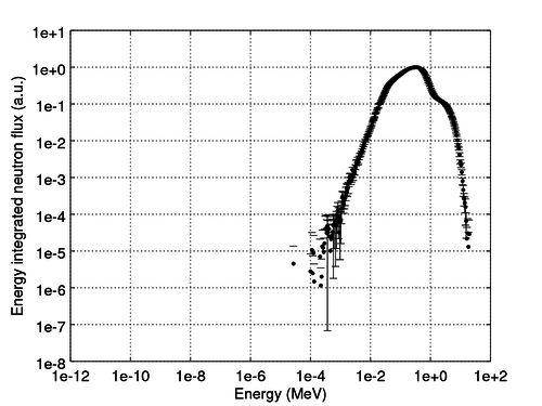
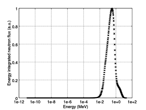
You can use the OCTAVE script below to plot the flux-spectrum.
Copy and paste the contents of the OCTAVE script to a file (you can name the file, e.g. analyze.m) in the same directory as infinite_det0.m and run it with OCTAVE:
octave analyze.m
This should produce figure files FluxEInt.png and FluxEIntLinY.png to the same directory.
The figures should look more or less like these:
We can see that the most of the neutron flux lies between 1e-2 and 1e1 MeV, which means that the system has a very fast neutron spectrum. As there are no light elements to work as neutron moderators, this is no surprise.
Testing the effect of added moderation
We can test how the addition of some light elements, e.g. hydrogen will affect the multiplication factor and flux spectrum of the system.
Starting from the (more or less) critical material definition
% --- Fuel material (5.76 wt-% enriched uranium), density 10.1 g/cm3

mat fuel     -10.1
92235.03c    -0.0576
92238.03c    -0.9424
we can add some hydrogen-1: The atomic number of hydrogen-1 is 1 and the mass number is also 1, which means that the basic part of the nuclide id will be 1001. We'll use the same library identifier as for the uranium, i.e. 03c:
% --- Fuel material (5.76 wt-% enriched uranium + some hydrogen), density 10.1 g/cm3
%     One part (in mass) of uranium, 0.005 parts (in mass) of hydrogen

mat fuel     -10.1
92235.03c    -0.0576
92238.03c    -0.9424
 1001.03c    -0.005
Here we have added 0.005 parts (in mass) of hydrogen-1 to our pre-existing 1.0 parts (in mass) of uranium. You may notice that the mass fractions now sum up to more than 1.0. In such situations Serpent will automatically normalize the mass-fractions so that they add up to 1.0.
Now you can run the simulation again.
You should notice that the multiplication factor is much higher this time, indicating that the addition of moderating material to the system increased the reactivity of the system.
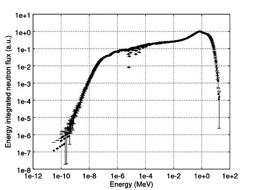
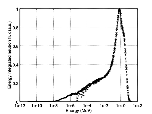
By running the OCTAVE script again, you can plot the flux-spectrum from the moderated system to obtain something like this:
Comparing these plots to the previous ones shows that the moderated system is more thermal, i.e. has higher neutron flux at the thermal energies than the unmoderated one.
Ideas for additional testing and tinkering in part 1
Remove the added hydrogen from your fuel material before moving to these additional tasks so that your system should be critical again (k-eff of approximately 1.0).
- Test the effect of unresolved resonance probability table sampling on the multiplication factor and flux spectrum of the critical fast system (set ures 1). The probability table sampling should be always set on for the simulation of fast systems. Do you see an effect on the running time? You can remove the set ures 1 before moving to the next part.
- Test changing the limiting surface s1 from type inf to one of the other surface types. For example, what is the multiplication factor of a cube centered at the origin (0, 0, 0) with a side-length of 10 cm cube (surface type cube, see also the input syntax for the surf command word)? Note: The unit of length in Serpent is cm. How large does the cube have to be to be considered infinite (i.e. to get the same k-eff as in the infinite system)?
- Modify the input so that you have a cube with a side length of 200 cm surrounded by a 10 cm cubic layer of heavy water. You'll need to add a second cuboid surface and one more cell definition. You can use the material definition below for the heavy water. What is the multiplication factor? How thick does the heavy water layer need to be for the system to be critical?
% --- Heavy water (density 1.11 g/cm3)
%     2 parts (atomic) of hydrogen-2, 1 parts (atomic) of oxygen-16
%     Hydrogen 2 is flagged as a bound scatterer with the "moder"-card

mat heavywater -1.11 moder MyThermLib 1002
 1002.03c       2
 8016.03c       1

% --- Define thermal scattering libraries associated with hydrogen-2

therm MyThermLib hwj3.00t
Part 2: A 2D pin-cell (infinite lattice)
Part 2 overview
The second model we shall use is a 2 dimensional pin-cell model (i.e. an infinite square lattice of fuel pins). The geometry is infinite both axially and radially.
We will use this model to familiarize ourselves with the geometry and mesh-plotter capabilities in Serpent and to calculate some radial reaction rate distributions in the fuel pellet of the pin.
You can create a new folder, where you put all the files of this pin-cell model.
Part 2 input
Copy and paste the input below to a file named pin on your computer.
Colors in the input correspond to:
- Comments
- Control words
- Name definitions
- Name references
Plotting the input
Before running a neutron transport simulation, it is typically a good idea to plot the geometry to verify that it has been defined correctly. The basics of geometry, track and mesh plotting are explained on a separate wiki page.
It is possible to execute only the geometry plotter, without running the neutron transport by using the command line argument -plot
sss2 -plot pin
Do this now. This will produce three plot files pin_geom1.png, pin_geom2.png, pin_geom3.png, which should look like the ones below:
You will probably notice that the colors in your geometry plots are a bit different from the ones shown above. If the user does not define a color for a material, Serpent will use a random color. Let's specify the colors for our materials using the rgb card. Add the bold rgb-definitions to the material definitions in your pin file:
% --- Fuel material (3.0 wt-% enriched uranium dioxide), density 10.1 g/cm3</span>

mat fuel     -10.1 rgb 240 240 100
92235.03c    -0.02644492
92238.03c    -0.85505247
 8016.03c    -0.11850261

% --- Cladding material for fuel rod
%     (100 % natural zirconium)

mat clad     -6.55 rgb 150 150 150
40000.03c    -1.0

% --- Water at 1.0 g/cm3
%     Defined using atomic fractions for the composition.
%     Hydrogen is flagged as a bound scatterer with the "moder"-card

mat water    -1.0 moder MyThermLib 1001 rgb 200 200 255
 1001.03c     2.0
 8016.03c     1.0
The rgb card is followed by three integer values between 0-255 for red, green and blue respectively. The ordering of additional cards in the material definition (e.g. the moder and the rgb cards) is interchangeable.
Re-plot the figures after defining the material colors. This should produce the same plots as previously, but with colors as below:
It is often a good idea to define easily distinguishable colors for each material so that they can be identified from the geometry plots. This makes it easier to spot cases, where the wrong material is used in a wrong place. Certain RGB-colors are used by Serpent to indicate specific problems with the geometry:
| RGB value | Color | Description |
|---|---|---|
| (0, 0, 0) | COLOR | Outside cell or void-material. |
| (0, 255, 0) | COLOR | No cell found at coordinates. |
| (255, 0, 0) | COLOR | Overlap of multiple cells found at coordinates. |
| (255, 0, 255) | COLOR | Undefined material density factor at coordinates. |
Running the input
Simply run the input from terminal, by being in the same directory as the input-file and executing
sss2 [-omp N] pin
the simulation should, again, produce multiple output files. This time a mesh-plot (pin_mesh1.png) is also produced:
The colour scheme of the mesh-plot consists of “hot” shades of red and yellow, representing relative fission power, and “cold” shades of blue, representing relative thermal flux (flux below 0.625 eV). As the mesh-plot is produced by a Monte Carlo simulation it is subject to statistical noise. The amount of statistical noise can be reduced by simulating more neutrons.
Setting up additional mesh-plots
The basic mesh-plot produced by Serpent shows the relative fission power distribution and the relative thermal flux distribution. Using detectors, it is possible to obtain a mesh-plot of many different distributions.
Let's calculate some of the reaction rate distributions by setting up detectors and linking them to additional mesh-plots:
% --- Detector that calculates the elastic scattering reaction rate in the system
%     Name of the detector is elastic.
%     The detector uses response number -3 (total elastic scattering cross section)
%     of the material at the interaction site (keyword: void)

det elastic dr -3 void

% --- A meshplot that shows the value of a detector response throughout the geometry (type 8)
%     The colormap that is used is "cold" (colormap 2)
%     The detector linked to this meshplot is named "elastic"
%     Orientation is xy (3), and output size is 200 by 200 pixel

mesh 8 2 elastic 3  200  200

% --- Detector that calculates the capture reaction rate in the system
%     Name of the detector is capture.
%     The detector uses response number -2 (total capture cross section)
%     of the material at the interaction site (keyword: void)

det capture dr -2 void

% --- A meshplot that shows the value of a detector response throughout the geometry (type 8)
%     The colormap that is used is "cold" (colormap 2)
%     The detector linked to this meshplot is named "capture"
%     Orientation is xy (3), and output size is 200 by 200 pixel

mesh 8 2 capture 3  200  200
Adding the new detector and mesh-plot definitions to the input file and re-running the simulation, will produce two additional mesh-plots:
The left figure shows the elastic scattering distribution, whereas the right figure shows the capture distribution. Darker colors indicate lower values and lighter colors indicate higher values.
Based on the two mesh-plots it is easy to see that the elastic scattering density is at its highest in water, whereas the capture density is at its highest in the fuel.
If the user does not define otherwise, the detectors will sum up responses from all materials, from all neutron energies and from all parts of the geometry. By using additional cards, the integration domain of the detector can be limited for example to include only specific materials (dm), energies (de), geometry cells (dc) or certain spatial coordinate ranges (dx, dy, dz). All of the available detector cards are detailed in the input syntax manual.
We can showcase these capabilities by modifying the capture rate detector to only include scores in the fuel-material:
% --- Detector that calculates the capture reaction rate in the fuel material
%     Name of the detector is capture.
%     The detector uses response number -2 (total capture cross section)
%     of the material at the interaction site (keyword: void)
%     Only scores interactions in material "fuel"

det capture dr -2 void dm fuel
Running the simulation again with the updated capture detector will result in a slightly different mesh-plot from the capture detector:
As the water material is no longer part of the scoring domain of the detector, the capture distribution in the fuel material is shown in greater contrast. We are now able to see that the capture rate is at its highest at the outer surface of the fuel material.
Calculating radial reaction rate distributions in the fuel pellet
The mesh-plots only show the relative values of the plotted distributions, which means that they are well suited for illustrating the shapes of the different distributions but do not provide any information on the absolute magnitude of the distributions.
In order to calculate the magnitudes (numerical values), detectors need to be set up with a suitable spatial binning. In order to calculate the radial fission and capture rate distributions in the fuel pellet, we will use a cylindrical binning for the detectors (add these to your pin-file):
% --- Detector that calculates the radial fission distribution in the fuel:
%     Name of the detector is RadialFission.
%     The detector uses response number -6 (total fission cross section)
%     of the material at the interaction site (keyword: void)
%     Detector only scores interactions at material "fuel" ("dm fuel").
%     Detector calculates the spatial distribution using a cylindrical mesh "dn 1"
%     with 20 bins in the radial direction between 0.0 and 0.4025 cm ("0.0 0.4025 20")
%     with 1 bin in the angular direction between 0 and 360 degrees ("0 360 1")
%     with 1 bin in the axial direction that extends from -infinity to infinity ("0 0 1")

det RadialFission dr -6 void dm fuel dn 1 0.0 0.4025 20 0 360 1 0 0 1

% --- Detector that calculates the radial capture distribution in the fuel:
%     Name of the detector is RadialCapture.
%     The detector uses response number -2 (total capture cross section)
%     of the material at the interaction site (keyword: void)
%     Detector only scores interactions at material "fuel" ("dm fuel").
%     Detector calculates the spatial distribution using a cylindrical mesh "dn 1"
%     with 20 bins in the radial direction between 0.0 and 0.4025 cm ("0.0 0.4025 20")
%     with 1 bin in the angular direction between 0 and 360 degrees ("0 360 1")
%     with 1 bin in the axial direction that extends from -infinity to infinity ("0 0 1")

det RadialCapture dr -2 void dm fuel dn 1 0.0 0.4025 20 0 360 1 0 0 1
If we want to obtain absolute values for the fission rate or capture rate we will also have to specify a normalization for our calculation. We will set the power level of our pin-cell to a 200 W/cm linear power (add this to your pin-file):
% --- Set system linear power to 200 W/cm (this is a 2D system)

set power 200
As you run the simulation again, you will obtain a detector file pin_det0.m containing the output from the RadialFission and RadialCapture detectors. You can use the OCTAVE script below (you'll need to expand the element on this page to see the code) to calculate and plot radial reaction rate density distributions based on the detector-output. I.e. save the contents of the OCTAVE script to a new file called analyzePin.m in the same folder as pin_det0.m and run the script with OCTAVE.
OCTAVE script for plotting radial reaction rate distributions. Save to analyzePin.m
#########################################
## Initial checking and pre-processing ##
#########################################

## Check that the detector file exists

if (exist("./pin_det0.m", "file") != 2)
  disp("Could not find pin_det0.m from current folder! Cannot do analysis.")
  exit()
endif

## Run the detector output file to bring the results to workspace

run pin_det0.m;

## Check that the detector outputs exist

if (exist("DETRadialFission", "var") != 1)
  disp("Could not find results for RadialFission from the detector\
 file (maybe misspelled detector name?). Cannot do analysis.")
  exit()
endif

## Check that the detector outputs exist

if (exist("DETRadialCapture", "var") != 1)
  disp("Could not find results for RadialCapture from the detector\
 file (maybe misspelled detector name?). Cannot do analysis.")
  exit()
endif

################################################################################
################################################################################
## Plot the radial fission rate distribution ###################################
################################################################################
################################################################################

## Get values for radial bins

val = DETRadialFission(:,11);

## Get relative errors

relerr = DETRadialFission(:,12);

## Get minimum radius of each bin

r0 = DETRadialFissionR(:,1);

## Get maximum radius of each bin

r1 = DETRadialFissionR(:,2);

## Calculate area of each bin

A = pi*(r1.^2-r0.^2);

## Divide values by area to get average fission density from fission

val = val./A;

## Calculate absolute errors for the fission density

abserr = val.*relerr;

##########################
## open figure and plot ##
##########################

figure('visible','off');

## Draw each bin separately

hold on;

for i=1:1:size(val,1)

  ## Draw horizontal line for the mean fission density of the bin

  plot([r0(i) r1(i)], [val(i) val(i)], 'k-', 'LineWidth', 2)

  ## Draw error estimates:

  ## Mean - 2*sigma

  plot([r0(i) r1(i)], [1 1]*(val(i) - abserr(i)*2), 'r-')

  ## Mean + 2*sigma

  plot([r0(i) r1(i)], [1 1]*(val(i) + abserr(i)*2), 'r-')

  ## Draw some vertical lines to make the plot nicer

  if (i > 1)
    ## For mean:

    plot([1 1]*r0(i), [val(i-1) val(i)], 'k-', 'LineWidth', 2)

    ## For mean - 2*sigma

    plot([1 1]*r0(i), [val(i-1)-abserr(i-1)*2 val(i)-abserr(i)*2], 'r-')

    ## For mean + 2*sigma

    plot([1 1]*r0(i), [val(i-1)+abserr(i-1)*2 val(i)+abserr(i)*2], 'r-')
  end

end

## Set axes

set(gca,'FontSize',16);

## Make the plot a bit nicer

xlim([0 0.45])
xlabel('Radius (cm)')
ylabel('Fission rate density (fissions/(s*cm3))')
grid on
grid minor off
box on

## Save the figure

print -dpng RadFiss.png;

## Close all figures

close all;

################################################################################
################################################################################
## Plot the radial capture rate distribution ###################################
################################################################################
################################################################################

## Get values for radial bins

val = DETRadialCapture(:,11);

## Get relative errors

relerr = DETRadialCapture(:,12);

## Get minimum radius of each bin

r0 = DETRadialCaptureR(:,1);

## Get maximum radius of each bin

r1 = DETRadialCaptureR(:,2);

## Calculate area of each bin

A = pi*(r1.^2-r0.^2);

## Divide values by area to get average capture density from capture

val = val./A;

## Calculate absolute errors for the capture density

abserr = val.*relerr;

##########################
## open figure and plot ##
##########################

figure('visible','off');

## Draw each bin separately

hold on;

for i=1:1:size(val,1)

  ## Draw horizontal line for the mean capture density of the bin

  plot([r0(i) r1(i)], [val(i) val(i)], 'k-', 'LineWidth', 2)

  ## Draw error estimates:

  ## Mean - 2*sigma

  plot([r0(i) r1(i)], [1 1]*(val(i) - abserr(i)*2), 'r-')

  ## Mean + 2*sigma

  plot([r0(i) r1(i)], [1 1]*(val(i) + abserr(i)*2), 'r-')

  ## Draw some vertical lines to make the plot nicer

  if (i > 1)
    ## For mean:

    plot([1 1]*r0(i), [val(i-1) val(i)], 'k-', 'LineWidth', 2)

    ## For mean - 2*sigma

    plot([1 1]*r0(i), [val(i-1)-abserr(i-1)*2 val(i)-abserr(i)*2], 'r-')

    ## For mean + 2*sigma

    plot([1 1]*r0(i), [val(i-1)+abserr(i-1)*2 val(i)+abserr(i)*2], 'r-')
  end

end

## Set axes

set(gca,'FontSize',16);

## Make the plot a bit nicer

xlim([0 0.45])
xlabel('Radius (cm)')
ylabel('Capture rate density (captures/(s*cm3))')
grid on
grid minor off
box on

## Save the figure

print -dpng RadCapt.png;
Running the OCTAVE script should produce two figure files RadCapt.png and RadFiss.png that resemble the ones shown here:
As stated before, all of the results obtained from a Monte Carlo simulation are statistical estimates. This is also illustrated in the plots: the black line is based on the mean value of the tallied reaction rate, whereas the red lines correspond to the mean +- 2 standard deviations.
Looking at the plots we can see that:
- Both the capture rate density and the fission rate density are at their highest at the outer surface of the pellet. This is due to flux self-shielding effects.
- The difference between pellet centerline and pellet surface reaction rate densities is larger for the capture rate density.
- More fissions than captures occur in the fuel.
- The statistical uncertainties are larger at the pellet centerline than at the pellet surface. This is explained mostly by the fact that the width of the radial bins is equal, which leads to the area (volume) of the radial bins being larger near the surface of the pellet than in the inner parts. A larger bin will, all other things being equal, tally more interactions, which leads to better statistics (smaller statistical uncertainties).
The statistical uncertainties can be reduced by simulating more neutrons, i.e. by increasing the number of neutrons per cycle or the number of active cycles in the set pop definition:
% --- Neutron population: 5000 neutrons per cycle, 100 active / 20 inactive cycles

set pop 5000 100 20
Ideas for additional testing and tinkering in part 2
- Try setting the boundary condition to vacuum (set bc 1) instead of reflective. How does the second geometry plot change? What happens to the multiplication factor? Why?
- Try increasing the number of radial bins for the RadialFission and RadialCapture detectors to e.g. 200. You can compare the shapes of the distributions and the statistical uncertainties to the previously calculated ones.
- Try running a simulation with more neutrons to see the effect on mesh-plots and detector results.
Part 3: A 2D assembly model (infinite lattice)
Part 3 overview
In the third part of the tutorial you will be working with a two dimensional model for one of the assembly types in an initial core loading of an EPR reactor[1].
The assembly contains 264 fuel rods, 20 of which have burnable absorber (Gd2O3) intermixed in the fuel. The assembly also contains 24 control rod guide tubes and one central instrumentation thimble. The geometry of the assembly is shown below. The yellow rods contain uranium dioxide fuel with 3.0 wt-% enrichment, whereas the green rods contain uranium dioxide fuel with a 0.25 wt-% enrichment and 8.0 wt-% Gd2O3 as a burnable absorber.
You can create a new folder, where you put all the files of this assembly model.
Part 3 input
Copy and paste the input below to a file named assembly on your computer.
Colors in the input correspond to:
- Comments
- Control words
- Name definitions
- Name references
Input for 2D assembly geometry
% --- Simple 2D EPR assembly geometry for Serpent tutorial

/************************
 * Material definitions *
 ************************/

% --- 3.0 wt-% enriched UO2
%     Temperature is set to 950 K

mat fuelNoGad  -10.3070 tmp 950.0 rgb 255 255 150
92235.09c       -0.02644492
92238.09c       -0.85505247
 8016.09c       -0.11850261

% --- 0.25 wt-% enriched UO2 with 8.0 wt-% of Gd2O3
%     Temperature is set to 650 K

mat fuelYesGad -10.3070 tmp 650.0 rgb 150 255 150
92235.06c       -0.00202753
92238.06c       -0.80898345
 8016.06c       -0.11957908
64152.06c       -0.00013411
64154.06c       -0.00148108
64155.06c       -0.01012049
64156.06c       -0.01408805
64157.06c       -0.01083999
64158.06c       -0.01731511
64160.06c       -0.01543111

% --- Cladding material Zircaloy-4
%     [Composition from PNNL-15870, Rev. 1]

mat Zircaloy4 -6.56000E+00 tmp 610
 8016.03c  -1.19276E-03
24050.03c  -4.16117E-05
24052.03c  -8.34483E-04
24053.03c  -9.64457E-05
24054.03c  -2.44600E-05
26054.03c  -1.12572E-04
26056.03c  -1.83252E-03
26057.03c  -4.30778E-05
26058.03c  -5.83334E-06
40090.03c  -4.97862E-01
40091.03c  -1.09780E-01
40092.03c  -1.69646E-01
40094.03c  -1.75665E-01
40096.03c  -2.89038E-02
50112.03c  -1.27604E-04
50114.03c  -8.83732E-05
50115.03c  -4.59255E-05
50116.03c  -1.98105E-03
50117.03c  -1.05543E-03
50118.03c  -3.35688E-03
50119.03c  -1.20069E-03
50120.03c  -4.59220E-03
50122.03c  -6.63497E-04
50124.03c  -8.43355E-04

% --- Coolant is water with 650 ppm soluble boric acid added
%     The temperature of water is 583 K
%     Density is calculated based on a pressure of 15.5 MPa
%     Hydrogen is flagged as a bound scatterer with the "moder"-card

mat water -0.70602 tmp 583 moder lwtr 1001 rgb 200 200 255
O-16.03c   3.330861e-01
H-1.03c    6.663259e-01
B-10.03c   7.186970e-05
B-11.03c   2.892846e-04

% --- Define thermal scattering libraries associated with hydrogen in light water
%     As there are no readymade thermal scattering libraries for 583 K
%     We will tell Serpent to interpolate using two bounding libraries:
%     -lwj3.11t (H-1 in light water at 574 K)
%     -lwj3.13t (H-1 in light water at 624 K)
%     See also: http://montecarlo.vtt.fi/download/SSS_THERMAL.pdf

therm lwtr 583 lwj3.11t lwj3.13t

/************************
 * Geometry definitions *
 ************************/

% --- Normal fuel rod (no gadolinia in fuel)

pin FF
fuelNoGad  0.3975
void       0.4125
Zircaloy4  0.4750
water

% --- Gadolinium fuel rod

pin GG
fuelYesGad  0.3975
void        0.4125
Zircaloy4   0.4750
water

% --- Empty instrumentation thimble

pin ii
water       0.5725
Zircaloy4   0.6125
water

% --- Empty control rod channel

pin cc
water       0.5725
Zircaloy4   0.6125
water

% --- Empty lattice position (just water)

pin ww
water

% --- Pin lattice definition, name of the lattice "lat1"
%     Lattice type 1 (square lattice)
%     Lattice centered at 0.0 0.0
%     19 x 19 lattice elements (17x17 fuel rods + 1 layer of water)
%     Lattice pitch 1.26 cm
%     We'll utilize our knowledge of the 1/8 symmetry so that
%     we'll only have to type in 1/8th of the assembly

lat lat1 1 0.0 0.0 19 19 1.26
ww ww ww ww ww ww ww ww ww ww ww ww ww ww ww ww ww ww ww
ww ww ww ww ww ww ww ww ww FF FF FF FF FF FF FF FF FF ww
ww ww ww ww ww ww ww ww ww FF FF FF FF FF FF FF FF ww ww
ww ww ww ww ww ww ww ww ww cc FF FF cc FF FF GG ww ww ww
ww ww ww ww ww ww ww ww ww FF GG FF FF FF cc ww ww ww ww
ww ww ww ww ww ww ww ww ww FF FF FF FF GG ww ww ww ww ww
ww ww ww ww ww ww ww ww ww cc FF FF cc ww ww ww ww ww ww
ww ww ww ww ww ww ww ww ww FF FF GG ww ww ww ww ww ww ww
ww ww ww ww ww ww ww ww ww FF FF ww ww ww ww ww ww ww ww
ww ww ww ww ww ww ww ww ww ii ww ww ww ww ww ww ww ww ww
ww ww ww ww ww ww ww ww ww ww ww ww ww ww ww ww ww ww ww
ww ww ww ww ww ww ww ww ww ww ww ww ww ww ww ww ww ww ww
ww ww ww ww ww ww ww ww ww ww ww ww ww ww ww ww ww ww ww
ww ww ww ww ww ww ww ww ww ww ww ww ww ww ww ww ww ww ww
ww ww ww ww ww ww ww ww ww ww ww ww ww ww ww ww ww ww ww
ww ww ww ww ww ww ww ww ww ww ww ww ww ww ww ww ww ww ww
ww ww ww ww ww ww ww ww ww ww ww ww ww ww ww ww ww ww ww
ww ww ww ww ww ww ww ww ww ww ww ww ww ww ww ww ww ww ww
ww ww ww ww ww ww ww ww ww ww ww ww ww ww ww ww ww ww ww

% --- Tell Serpent to apply a symmetry to the lattice "lat1"
%     Symmetry axis is the z-axis (3)
%     Symmetry boundary condition is reflective (2)
%     Symmetry axis is located at coordinates (0.0 0.0)
%     Symmetry covers an angle starting from 270 degrees
%     and extending for 45 degrees

set usym lat1 3 2 0.0 0.0 270 45

% --- A square surface around the fuel assembly

surf s1 sqc  0.0 0.0 10.752

% --- Cell c1 belongs to the base universe 0, is filled with the lattice lat1
%     and covers everything inside surface s1

cell c1 0 fill lat1     -s1

% --- Cell c2 belongs to the base universe 0, is defined as an "outside" cell
%     and covers everything outside surface s1

cell c2 0 outside        s1

/******************
 * Run parameters *
 ******************/

% --- Assembly linear power is 420 kW

set power 42000

% --- Boundary condition (1 = black, 2 = reflective, 3 = periodic)

set bc 2

% --- Neutron population: 10000 neutrons per cycle, 100 active / 20 inactive cycles

set pop 10000 100 20

% --- XY-plot (3), which is 700 by 700 pixels and covers the whole geometry

plot 3 700 700

% --- XY-meshplot (3), which is 700 by 700 pixels and covers the whole geometry

mesh 3 700 700
Running the input for the assembly geometry
Simply run the input from terminal, by being in the same directory as the input-file and executing
sss2 [-omp N] assembly
the simulation should, again, produce multiple output files and also the geometry and mesh-plots:
Based on the mesh-plot, we can see that the fission power is much lower in the fuel rods that contain the burnable absorber (BA) than in the normal fuel rods. The BA-rods also create a depression (decrease) in the thermal flux distribution in their immediate surroundings.
Increasing the number of simulated neutrons will increase the simulation time, but reduce the statistical noise in the mesh-plot. For example, simulating 15000 active cycles with 20000 neutrons in each cycle will result in this:
Testing the power feedback effects in the assembly
One important part of safe reactor design is to ensure that the power reactivity feedbacks for the reactor are negative in the operating conditions. This means that changes that follow from increased reactor power (such as increase in fuel and coolant/moderator temperature) decrease the multiplication factor of the system.
We will test the negativity of these feedbacks in our fuel assembly model.
Make a note of the multiplication factor you obtained from the first simulation, for example:
k-eff (implicit) = 0.98086 +/- 0.00069 [0.97950 0.98222]
Let's assume that an increase in reactor power will bring about the following changes in material temperatures and densities:
- Fuel temperature for non-burnable absorber rods will increase by 300 K.
- Fuel temperature for burnable absorber rods will increase by 50 K.
- Moderator temperature will increase by 25 K.
- Moderator density will decrease to 0.635 g/cm3.
We'll calculate the effects these changes have on the multiplication factor of our assembly. The next subsections will give information on how to apply these changes to the input.
Changing the fuel temperature
For the fuel materials we can simply change the value in the tmp card in the material definition.
For the non-gadolinia fuel we will change the definition to
mat fuelNoGad  -10.3070 tmp 1250.0 rgb 255 255 150
92235.09c       -0.02644492
92238.09c       -0.85505247
 8016.09c       -0.11850261
And for the gadolinia containing fuel we will use
mat fuelYesGad -10.3070 tmp 700.0 rgb 150 255 150
92235.06c       -0.00202753
92238.06c       -0.80898345
 8016.06c       -0.11957908
64152.06c       -0.00013411
64154.06c       -0.00148108
64155.06c       -0.01012049
64156.06c       -0.01408805
64157.06c       -0.01083999
64158.06c       -0.01731511
64160.06c       -0.01543111
Changing the water temperature
For the water temperature change, we'll need to modify both the value in the tmp card of the material definition and the value in the therm definition:
mat water -0.70602 tmp 608 moder lwtr 1001 rgb 200 200 255
O-16.03c   3.330861e-01
H-1.03c    6.663259e-01
B-10.03c   7.186970e-05
B-11.03c   2.892846e-04
and
therm lwtr 608 lwj3.11t lwj3.13t
Changing the water density
For the water density change, it is enough to change the mass density given in the material definition:
mat water -0.635 tmp 608 moder lwtr 1001 rgb 200 200 255
O-16.03c   3.330861e-01
H-1.03c    6.663259e-01
B-10.03c   7.186970e-05
B-11.03c   2.892846e-04
Calculating the k-eff for the modified system
After applying all of the changes to your input, you can run the simulation again to see the effect on the multiplication factor. Make a note of the new multiplication factor, e.g.
k-eff (implicit) = 0.96574 +/- 0.00073 [0.96430 0.96718]
Comparing the new multiplication factor to the previously obtained we see that our modifications resulted in a clear decrease in the multiplication factor: It went from 0.98086 +/- 0.00069 to 0.96574 +/- 0.00073. The feedback effect seems to be negative in our assembly, as it should be.
Calculating the pin power distribution
In safety analysis, the pin power distribution in each assembly is often a requested output from neutronics calculations. The pin power distribution helps in identifying the limiting fuel rod, i.e. the fuel rod with the highest fuel centerline temperature or highest heat flux at the cladding surface.
We'll use a simple mesh-detector to calculate the pin power distribution for our assembly:
% --- Detector that calculates the pin power distribution in the assembly:
%     Name of the detector is pinpowers.
%     The detector uses response number -8 (fission heat deposition)
%     of the material at the interaction site (keyword: void).
%     The detector has 17 bins in the x-direction between -10.71 cm and 10.71 cm
%     The detector has 17 bins in the y-direction between -10.71 cm and 10.71 cm

det pinpowers dr -8 void dx -10.71 10.71 17 dy -10.71 10.71 17
Add the detector definition to your input and run the calculation again. The calculation will now produce the detector output file assembly_det0.m that contains the results for our newly defined detector. You can use the OCTAVE script below (you'll need to expand the element on this page to see the code) to calculate and plot radial reaction rate density distributions based on the detector-output. I.e. save the contents of the OCTAVE script to a new file called analyzeAssembly.m in the same folder as assembly_det0.m and run the script with OCTAVE.
OCTAVE script for plotting pin power distribution. Save to analyzeAssembly.m
#########################################
## Initial checking and pre-processing ##
#########################################

## Check that the detector file exists

if (exist("./assembly_det0.m", "file") != 2)
  disp("Could not find assembly_det0.m from current folder! Cannot do analysis.")
  exit()
endif

## Run the detector output file to bring the results to workspace

run assembly_det0.m;

## Check that the detector outputs exist

if (exist("DETpinpowers", "var") != 1)
  disp("Could not find results for pinpowers from the detector\
 file (maybe misspelled detector name?). Cannot do analysis.")
  exit()
endif

#####################################
## Plot the pin power distribution ##
#####################################

## Get values for pin powers

val = DETpinpowers(:,11);

## Remove zero-values (control rod channels)

val(val==0) = NaN;

## Get relative errors

relerr = DETpinpowers(:,12);

## Reshape the arrays

val    = reshape(val, [17, 17]);
relerr = reshape(relerr, [17, 17]);

## Calculate absolute errors

abserr = val.*relerr*2;

##########################
## open figure and plot ##
##########################

figure('visible','off');

## 2D color plot of the values

imagesc(val);

## Change the color scheme to something better

colormap("autumn");

## Add a colorbar

cb = colorbar();

## Tune the colorbar and label text

set(cb, 'FontSize',16);
set(cb, 'Ylabel', 'Linear power (W/cm)');
h = get(cb, 'YLabel');
set(h, 'FontSize',16);

## Add numbers for each rod

for i=1:1:17
  for j=1:1:17

    ## Calculate x and y position for the text of current rod

    x    = i-0.35 ;
    y    = j-0.2;
    xerr = i-0.46;
    yerr = j+0.2;

    ## Get current rod linear power (rounded to W/cm)

    curval = round(val(i,j));
    curerr = round(abserr(i,j)*10)/10;

    ## Add text for current rod

    if (! isnan(curval))

      ## Linear power

      text(x, y, num2str(curval), 'FontSize', 7);

      ## +- 2*sigma uncertainty

      text(xerr, yerr, ["+- " num2str(curerr)], 'FontSize', 7);

    endif
  endfor

  ## Add some lines to make the picture nicer

  line([0.5 17.5], [i i]+0.5);
  line([i i]+0.5, [0.5 17.5]);

endfor

## Make the plot a bit nicer by removing the tick-marks

set(gca, 'XTick', []);
set(gca, 'YTick', []);

## Add title to the plot

title("Pin power distribution (linear powers +- 2*sigma uncertainty)")

## Save the figure

print -dpng PinPowers.png;

## Close all figures

close all;
Running the OCTAVE script should produce a figure file PinPowers.png that resembles the one shown here:
The figure shows the linear power of each pin by color and as text. The maximum linear powers are around 180 W/cm and are located in the lattice positions both at the assembly outer boundary and around the central instrumentation thimble. The linear power of the burnable absorber rods is significantly lower, approximately 14W/cm.
Even though the assembly is symmetric, the power distribution is not exactly symmetric. This is again due to the statistical nature of Monte Carlo transport. Typically one can average the results from symmetrical lattice positions as a part of the post processing to obtain a symmetric distribution.
Ideas for additional testing and tinkering in part 3
Part 4: Assembly burnup calculation
Part 4 overview
In this part of the tutorial you will conduct a burnup (depletion) calculation for the 2D assembly model presented previously.
You can create a new folder, where you put all the files of this assembly burnup calculation.
Part 4 input
The input is the same as in the previous part of the tutorial except for a few differences:
- The two fuel materials are flagged as burnable materials with the burn 1 card in the material definition.
- The temperature of fuelYesGd is also set to 950 K.
- The neutron population is reduced to 5000 neutrons per cycle, 100 active / 20 inactive cycles to reduce the calculation time.
- There are several new definitions under the title Settings for the burnup calculation in the end of the input file.
Copy and paste the input below to a file named burn on your computer.
Colors in the input correspond to:
- Comments
- Control words
- Name definitions
- Name references
Input for assembly burnup calculation
% --- Simple 2D EPR assembly geometry burnup model for Serpent tutorial

/************************
 * Material definitions *
 ************************/

% --- 3.0 wt-% enriched UO2
%     Temperature is set to 950 K

mat fuelNoGad  -10.3070 tmp 950.0 rgb 255 255 150 burn 1
92235.09c       -0.02644492
92238.09c       -0.85505247
 8016.09c       -0.11850261

% --- 0.25 wt-% enriched UO2 with 8.0 wt-% of Gd2O3
%     Temperature is set to 950 K

mat fuelYesGad -10.3070 tmp 950.0 rgb 150 255 150 burn 1
92235.09c       -0.00202753
92238.09c       -0.80898345
 8016.09c       -0.11957908
64152.09c       -0.00013411
64154.09c       -0.00148108
64155.09c       -0.01012049
64156.09c       -0.01408805
64157.09c       -0.01083999
64158.09c       -0.01731511
64160.09c       -0.01543111

% --- Cladding material Zircaloy-4
%     [Composition from PNNL-15870, Rev. 1]

mat Zircaloy4 -6.56000E+00 tmp 610
 8016.03c  -1.19276E-03
24050.03c  -4.16117E-05
24052.03c  -8.34483E-04
24053.03c  -9.64457E-05
24054.03c  -2.44600E-05
26054.03c  -1.12572E-04
26056.03c  -1.83252E-03
26057.03c  -4.30778E-05
26058.03c  -5.83334E-06
40090.03c  -4.97862E-01
40091.03c  -1.09780E-01
40092.03c  -1.69646E-01
40094.03c  -1.75665E-01
40096.03c  -2.89038E-02
50112.03c  -1.27604E-04
50114.03c  -8.83732E-05
50115.03c  -4.59255E-05
50116.03c  -1.98105E-03
50117.03c  -1.05543E-03
50118.03c  -3.35688E-03
50119.03c  -1.20069E-03
50120.03c  -4.59220E-03
50122.03c  -6.63497E-04
50124.03c  -8.43355E-04

% --- Coolant is water with 650 ppm soluble boric acid added
%     The temperature of water is 583 K
%     Density is calculated based on a pressure of 15.5 MPa
%     Hydrogen is flagged as a bound scatterer with the "moder"-card

mat water -0.70602 tmp 583 moder lwtr 1001 rgb 200 200 255
O-16.03c   3.330861e-01
H-1.03c    6.663259e-01
B-10.03c   7.186970e-05
B-11.03c   2.892846e-04

% --- Define thermal scattering libraries associated with hydrogen in light water
%     As there are no readymade thermal scattering libraries for 583 K
%     We will tell Serpent to interpolate using two bounding libraries:
%     -lwj3.11t (H-1 in light water at 574 K)
%     -lwj3.13t (H-1 in light water at 624 K)
%     See also: http://montecarlo.vtt.fi/download/SSS_THERMAL.pdf

therm lwtr 583 lwj3.11t lwj3.13t

/************************
 * Geometry definitions *
 ************************/

% --- Normal fuel rod (no gadolinia in fuel)

pin FF
fuelNoGad  0.3975
void       0.4125
Zircaloy4  0.4750
water

% --- Gadolinium fuel rod

pin GG
fuelYesGad  0.3975
void        0.4125
Zircaloy4   0.4750
water

% --- Empty instrumentation thimble

pin ii
water       0.5725
Zircaloy4   0.6125
water

% --- Empty control rod channel

pin cc
water       0.5725
Zircaloy4   0.6125
water

% --- Empty lattice position (just water)

pin ww
water

% --- Pin lattice definition, name of the lattice "lat1"
%     Lattice type 1 (square lattice)
%     Lattice centered at 0.0 0.0
%     19 x 19 lattice elements (17x17 fuel rods + 1 layer of water)
%     Lattice pitch 1.26 cm
%     We'll utilize our knowledge of the 1/8 symmetry so that
%     we'll only have to type in 1/8th of the assembly

lat lat1 1 0.0 0.0 19 19 1.26
ww ww ww ww ww ww ww ww ww ww ww ww ww ww ww ww ww ww ww
ww ww ww ww ww ww ww ww ww FF FF FF FF FF FF FF FF FF ww
ww ww ww ww ww ww ww ww ww FF FF FF FF FF FF FF FF ww ww
ww ww ww ww ww ww ww ww ww cc FF FF cc FF FF GG ww ww ww
ww ww ww ww ww ww ww ww ww FF GG FF FF FF cc ww ww ww ww
ww ww ww ww ww ww ww ww ww FF FF FF FF GG ww ww ww ww ww
ww ww ww ww ww ww ww ww ww cc FF FF cc ww ww ww ww ww ww
ww ww ww ww ww ww ww ww ww FF FF GG ww ww ww ww ww ww ww
ww ww ww ww ww ww ww ww ww FF FF ww ww ww ww ww ww ww ww
ww ww ww ww ww ww ww ww ww ii ww ww ww ww ww ww ww ww ww
ww ww ww ww ww ww ww ww ww ww ww ww ww ww ww ww ww ww ww
ww ww ww ww ww ww ww ww ww ww ww ww ww ww ww ww ww ww ww
ww ww ww ww ww ww ww ww ww ww ww ww ww ww ww ww ww ww ww
ww ww ww ww ww ww ww ww ww ww ww ww ww ww ww ww ww ww ww
ww ww ww ww ww ww ww ww ww ww ww ww ww ww ww ww ww ww ww
ww ww ww ww ww ww ww ww ww ww ww ww ww ww ww ww ww ww ww
ww ww ww ww ww ww ww ww ww ww ww ww ww ww ww ww ww ww ww
ww ww ww ww ww ww ww ww ww ww ww ww ww ww ww ww ww ww ww
ww ww ww ww ww ww ww ww ww ww ww ww ww ww ww ww ww ww ww

% --- Tell Serpent to apply a symmetry to the lattice "lat1"
%     Symmetry axis is the z-axis (3)
%     Symmetry boundary condition is reflective (2)
%     Symmetry axis is located at coordinates (0.0 0.0)
%     Symmetry covers an angle starting from 270 degrees
%     and extending for 45 degrees

set usym lat1 3 2 0.0 0.0 270 45

% --- A square surface around the fuel assembly

surf s1 sqc  0.0 0.0 10.752

% --- Cell c1 belongs to the base universe 0, is filled with the lattice lat1
%     and covers everything inside surface s1

cell c1 0 fill lat1     -s1

% --- Cell c2 belongs to the base universe 0, is defined as an "outside" cell
%     and covers everything outside surface s1

cell c2 0 outside        s1

/******************
 * Run parameters *
 ******************/

% --- Assembly linear power is 420 kW

set power 42000

% --- Boundary condition (1 = black, 2 = reflective, 3 = periodic)

set bc 2

% --- Neutron population: 5000 neutrons per cycle, 100 active / 20 inactive cycles

set pop 5000 100 20

% --- XY-plot (3), which is 700 by 700 pixels and covers the whole geometry

plot 3 700 700

% --- XY-meshplot (3), which is 700 by 700 pixels and covers the whole geometry

mesh 3 700 700

/***************************************
 * Settings for the burnup calculation *
 ***************************************/

% --- Burnup points for the burnup calculation (in MWd/kgU)
%     Too long intervals between the burnup points will decrease the
%     accuracy of the burnup calculation, especially during the burn-out
%     of burnable absorber

dep butot 0.1  0.5  1  3  5  7  9  11  13  15  17  19

% --- Material division for burnup calculation
%     Treat different pins of fuelNoGad as separate depletion zones (sep 1)

div fuelNoGad  sep 1

% --- Material division for burnup calculation
%     Treat different pins of fuelYesGad as separate depletion zones (sep 1)
%     additionally divide each of those fuel pellets into 10 equal volume rings
%     between radial coordinates of 0.0 and 0.3975

div fuelYesGad sep 1 subr 10 0.0 0.3975

% --- Calculate material volumes before simulation by
%     sampling 10 million random points in the geometry.
%     Specifying the material volumes is crucial in burnup calculations

set mcvol 10000000

% --- Nuclide inventory: these nuclides will be included in the
%     depletion output file burn_dep.m. The list can be changed
%     after the simulation has concluded if needed. Then you can run
%     sss2 -rdep burn
%     which will make Serpent re-read the inventory and re-produce the
%     depletion output file.

set inventory
 922350
 942390
 641550
 641570

% --- Use predictor corrector method for the depletion solution
%     leli: Linear extrapolation on predictor
%           Linear interpolation on corrector
%     10 10: 10 substeps on predictor, 10 substeps on corrector

set pcc leli 10 10

% --- Decay data library needs to be specified for burnup calculations

set declib "sss_jeff31.dec"

% --- Neutron induced fission yield library needs to be specified for
%     burnup calculations

set nfylib "sss_jeff31.nfy"

% --- Reduce unionized energy grid size in order to save some memory
%     Use grid thinning with 5e-5 reconstruction tolerance between
%     1e-9 and 15 MeV.

set egrid 5e-5 1e-9 15.0
Depletion zone division
In burnup calculations it is usually necessary to subdivide the materials into multiple depletion zones. This is due to the fact that even if the material composition is initially the same in multiple different fuel rods, the differences in the local neutron flux between, e.g. different lattice positions should produce different compositions for the depleted fuel. Similarly, fuel rods that contain burnable absorber should be divided into rings to accurately capture the radial burn-out of the absorber. Significant errors may be introduced to the results if materials are not correctly divided to depletion zones.
Serpent has an easy to use methodology for automatically dividing the materials into user specified depletion zones. This might be a good time to visit the wiki-page describing that capability: Automated depletion zone division
In the input above, all of the unique lattice positions are treated as a separate depletion zone and the burnable absorber rods are further subdivided into 10 rings of equal area using the div definitions:
% --- Material division for burnup calculation
%     Treat different pins of fuelNoGad as separate depletion zones (sep 1)

div fuelNoGad  sep 1

% --- Material division for burnup calculation
%     Treat different pins of fuelYesGad as separate depletion zones (sep 1)
%     additionally divide each of those fuel pellets into 10 equal volume rings
%     between radial coordinates of 0.0 and 0.3975

div fuelYesGad sep 1 subr 10 0.0 0.3975
Specifying material volumes
It is important to make certain that Serpent uses the correct material volumes in burnup calculations. Serpent will automatically try to estimate the material volumes for each input but this will only yield good results in simple 2D cases. This will fail for certain in any geometries containing symmetries in the fuel assemblies.
See: Defining material volumes
Usually it is best to check the material volumes using the
sss2 -checkvolumes POINTS input
command. In this example, we have told Serpent to sample 10 million random points in the geometry before the calculation to obtain a statistical estimate of the material volumes and use those volumes for the burnup calculation:
% --- Calculate material volumes before simulation by
%     sampling 10 million random points in the geometry.
%     Specifying the material volumes is crucial in burnup calculations

set mcvol 10000000
Using more points will yield more accurate estimates for the volumes but will take more time.
Running the burnup calculation
Run the burnup simulation, preferably using OpenMP parallelization (try e.g. N = 4) as the burnup calculations tend to take a long time:
sss2 -omp N burn
During the simulation, Serpent executes two neutron transport solutions for each burnup step, meaning that the whole simulation will take a while (30 minutes to several hours depending on computer and parallelization).
The simulation will produce a separate mesh-plot for each burnup point:
The mesh-plots show that the burnable absorber rods begin to produce some fission power as the burnable absorber is consumed from them. The maximum of the fission power distribution also seems to move to the inner parts of the assembly from the outer part during the fuel depletion.
The depletion results, e.g. the specified nuclide inventories, material specific burnups and nuclide inventories are printed into the output file burn_dep.m. The results from the neutron transport simulation at each burn up point (e.g. estimates for multiplication factor) are appended to the main results file burn_res.m.
Changes in assembly due to burnup
We can use the results produced by the simulation to analyze the evolution of the multiplication factor as well as the masses of some interesting nuclides during the burnup calculation.
You can use the OCTAVE script below (you'll need to expand the element on this page to see the code) to calculate and plot some burnup depended quantities based on the results of the burnup calculation. I.e. save the contents of the OCTAVE script to a new file called analyzeBurn.m in the same folder as burn_res.m and burn_dep.m and run the script with OCTAVE.
OCTAVE script for plotting burnup dependent results. Save to analyzeBurn.m
#########################################
## Initial checking and pre-processing ##
#########################################

## Check that the main results file exists

if (exist("./burn_res.m", "file") != 2)
  disp("Could not find burn_res.m from current folder! Cannot do analysis.")
  exit()
endif

## Check that the depletion output file exists

if (exist("./burn_dep.m", "file") != 2)
  disp("Could not find burn_dep.m from current folder! Cannot do analysis.")
  exit()
endif

## Run both of the files to bring the results to workspace

run burn_res.m;
run burn_dep.m;

###############################################
## Plot the multiplication factor vs. burnup ##
###############################################

figure('visible','off');
errorbar(BU, IMP_KEFF(:,1), IMP_KEFF(:,1).*IMP_KEFF(:,2)*2,'k.')

## Set font size for the axes

set(gca, 'FontSize',16);

## Add labels for the axes

xlabel("Burnup (MWd/kgU)");
ylabel("Multiplication factor");

## Add title to the plot

title("Multiplication factor of the assembly as a function of burnup")

## Set limits for the axes

xlim([0 20]);
ylim([0.95 1.05]);

## Make the plot a bit nicer

grid on;
box on;

## Save the figure

print -dpng Keff.png;

## Close all figures

close all;

###############################
## Plot U235 mass vs. burnup ##
###############################

figure('visible','off');
plot(BU, TOT_MASS(iU235, :), 'k.-')

## Set font size for the axes

set(gca, 'FontSize',16);

## Add labels for the axes

xlabel("Burnup (MWd/kgU)");
ylabel("U-235 mass (g/cm of axial height)");

## Add title to the plot

title("U-235 mass in the assembly as a function of burnup")

## Set limits for the axes

xlim([0 20]);
ylim([0 35]);

## Make the plot a bit nicer

grid on;
box on;

## Save the figure

print -dpng mU235.png;

################################
## Plot Pu239 mass vs. burnup ##
################################

figure('visible','off');
plot(BU, TOT_MASS(iPu239, :), 'k.-')

## Set font size for the axes

set(gca, 'FontSize', 16);

## Add labels for the axes

xlabel("Burnup (MWd/kgU)");
ylabel("Pu-239 mass (g/cm of axial height)");

## Add title to the plot

title("Pu-239 mass in the assembly as a function of burnup")

## Make the plot a bit nicer

grid on;
box on;

## Save the figure

print -dpng mPu239.png;

## Close all figures

############################################
## Plot Gd155 and Gd157 masses vs. burnup ##
############################################

figure('visible','off');
plot(BU, TOT_MASS(iGd155, :), 'b.-')
hold on
plot(BU, TOT_MASS(iGd157, :), 'r.-')
hold off

## Add a legend

h1 = legend("Gd-155", "Gd-157", "location", "northeast");

## Set font size for the legend

set(h1, "FontSize", 16);

## Set font size for the axes

set(gca, "FontSize", 16);

## Add labels for the axes

xlabel("Burnup (MWd/kgU)");
ylabel("Mass (g/cm of axial height)");

## Add title to the plot

title("Gd-155 and Gd-157 mass in the assembly as a function of burnup")

## Set limits for the axes

xlim([0 20]);
ylim([0 1.2]);

## Make the plot a bit nicer

grid on;
box on;

## Save the figure

print -dpng mGd.png;

## Close all figures

close all;
Running the script will produce four figure files:
- Keff.png: The multiplication factor of the assembly as a function of burnup.
- mGd.png: The masses of 155Gd and 157Gd isotopes in the assembly (per unit length) as a function of burnup.
- mU235.png: The mass of 235U in the assembly (per unit length) as a function of burnup.
- mPu239.png: The mass of 239Pu in the assembly (per unit length) as a function of burnup.
The Keff.png plot should resemble this one:
We can see that the initial multiplication factor is approximately 0.98 and it decreases sharply during the first step of the calculation. This is due to the production of neutron absorbing fission products (neutron poisons). The concentrations of these neutron absorbers soon reach an equilibrium and the multiplication factor does not decrease any more. On the contrary, the multiplication factor starts to increase due to the fact that the neutron absorbers in the burnable absorber rods (mainly 155Gd and 157Gd) are consumed (see the next picture: mGd.png). Between 11 and 13 Mwd/kgU the last of the burnable absorbers are removed and the multiplication factor does not increase any more. Instead, it begins to fall due to the consumption of the initial fissile isotope 235U (see mU235.png) although the fissile nuclide 239Pu is also produced from 238U (see mPu239.png).
The other figures should look like these:
- mGd.png:
- mU235.png:
- mPu239.png:
It should be noted that the nuclide densities printed in burn_dep.m are statistical estimates and thus contain a statistical uncertainty. However, the statistical uncertainty of the nuclide densities cannot be easily calculated inside the Serpent simulation and typically the best way to estimate this uncertainty is to execute the same burnup simulation many times (e.g. tens of times) using different random number seeds and looking at the differences in the resulting nuclide densities.
Ideas for additional testing and tinkering in part 4
Part 5: A 3D research reactor model
Part 5 overview
In this last part of the tutorial you will build a Serpent model for an imaginary low power pool-type research reactor core. The reactor is inspired partly by critical pin-lattice configurations and partly by the TRIGA research reactor type.
The (simplified) geometry of the reactor is shown below for an xy-cut at axial midplane of the core and xz-cuts at core center and at the control rods:
Below is the overview of the core:
- The core contains 493 fuel rods (length 50 cm) with 3.0 wt-% enriched fuel. The fuel rods are similar to the non burnable absorber rods used in the EPR example.
- The core contains four movable boron carbide control rods located symmetrically around the core.
- The core is reflected by a circular graphite reflector.
- The core is located in a light water pool.
- The core has two 2 cm thick steel grid plates with holes for the fuel rods and control rods. There are some empty positions where additional fuel rods could be added at the periphery of the core. The two grids are identical, with the top grid shown here:
The empty lattice positions can be seen as blue circles, whereas the lattice positions filled with fuel rods are seen in light grey. The positions of the four control rods are seen as dark grey circles, surrounded with light blue water.
Part 5 geometry details
Radial geometry
This section details the measures needed to build the geometry model for the core. The general radial geometry can be summarized as:
- The outer radius of the grid plates is 26 cm.
- The inner radius of the graphite reflector is 30 cm.
- The outer radius of the graphite reflector is 60 cm.
- The outer radius of the model is 100 cm.
Axial geometry
The height of the graphite reflector is 100 cm and it covers the active fuel height symmetrically.
- The bottom of the model is 100 cm below axial midplane.
- The bottom of the graphite reflector is 50 cm below axial midplane.
- The bottom of the lower grid plate is 37 cm below axial midplane, which is also the bottom of fuel rods and the bottom of the control rod guide tubes.
- The top of the lower grid plate is 35 cm below axial midplane.
- The bottom of active fuel is 25 cm below the axial midplane.
- The top of active fuel is 25 cm above the axial midplane.
- The bottom of of the upper grid plate is 30 cm above axial midplane
- The top of of the upper grid plate is 32 cm above axial midplane
- The top of of the fuel rods is 35 cm above axial midplane.
- The top of the graphite reflector is 50 cm above axial midplane.
- The top of the model is 100 cm above axial midplane.
Lattice and grid plate geometry
The core lattice is a square lattice with a lattice pitch of 1.8 cm. The grid plates contain 4 holes for control rods and 583 holes for fuel rods in a roughly circular shape. 493 of the fuel rod positions are filled with fuel rods. The core lattice exhibits a 1/8 (45 degree) symmetry.
- The outer radius of the grid plates is 26 cm.
- The radius of the control rod holes in the grid plates is 0.85 cm.
- The radius of the fuel rod holes in the grid plates is 0.485 cm.
Fuel rod geometry
The fuel rod geometry is shown below (contracted axially by a factor of 7).
The radial geometry of the active fuel part is as follows:
- Fuel pellet outer radius 0.3975 cm.
- Cladding inner radius 0.4125 cm.
- Cladding outer radius 0.4750 cm.
The region between the fuel pellet and cladding is filled with a fill gas, but can be modelled as void.
The end-plugs below and above the active fuel consist of solid cladding material and have an outer radius equal to the cladding outer radius (0.4750 cm).
Control rod geometry
The control rods move in their guide tubes and they consist axially of three parts:
- Bottom 12 cm is made of stainless steel.
- The absorber part is 50 cm long and made out of boron carbide (B4C).
- The top part is made of stainless steel and extends out of the reactor to the control rod drive system (not included in the model).
The outer radius of the control rods is a constant 0.60 cm for all of the axial parts.
The guide tubes extend from the bottom of the bottom plate to the top of the model and are normally filled with water. The guide tubes are made of Zircaloy-4 and their radial dimensions are given below:
- Guide tube inner radius 0.75 cm.
- Guide tube outer radius 0.80 cm.
The figures below show the control rods in their fully inserted and fully withdrawn positions. In the fully inserted position the absorber part of the control rods coincides with the active fuel part of the fuel rods. The travel distance between the fully inserted and fully withdrawn positions is 50 cm (the same as the absorber length).
Part 5 material details
The reactor contains six different materials:
- Uranium dioxide fuel with 3.0 wt-% enrichment and a density of 10.37 g/cm3.
- Zircaloy-4 as the cladding and guide tube material. Density 6.56 g/cm3.
- Normal light water (density 1.0 g/cm3) filling the reactor pool and guide tubes.
- Graphite (density 1.719 g/cm3) as a radial reflector.
- Boron carbide (B4C) as the control rod absorber material. Density 2.52 g/cm3.
- Stainless steel as the grid plates and in the non-absorbing part of the control rods. Density 8.0 g/cm3.
The material definitions are given below
Colors in the input correspond to:
- Comments
- Control words
- Name definitions
- Name references
Material definitions for research reactor. Copy to a file named materials.
/************************
 * Material definitions *
 ************************/

% --- 3.0 wt-% enriched uranium dioxide fuel
%     Density of the fuel 10.307 g/cm3.

mat fuel    -10.3070 rgb 255 255 150
92235.03c    -0.02644492
92238.03c    -0.85505247
 8016.03c    -0.11850261

% --- Cladding material Zircaloy-4
%     [Composition from PNNL-15870, Rev. 1]
%     Density 6.56 g/cm3

mat Zircaloy4 -6.56000E+00 rgb 200 200 200
 8016.03c     -1.19276E-03
24050.03c     -4.16117E-05
24052.03c     -8.34483E-04
24053.03c     -9.64457E-05
24054.03c     -2.44600E-05
26054.03c     -1.12572E-04
26056.03c     -1.83252E-03
26057.03c     -4.30778E-05
26058.03c     -5.83334E-06
40090.03c     -4.97862E-01
40091.03c     -1.09780E-01
40092.03c     -1.69646E-01
40094.03c     -1.75665E-01
40096.03c     -2.89038E-02
50112.03c     -1.27604E-04
50114.03c     -8.83732E-05
50115.03c     -4.59255E-05
50116.03c     -1.98105E-03
50117.03c     -1.05543E-03
50118.03c     -3.35688E-03
50119.03c     -1.20069E-03
50120.03c     -4.59220E-03
50122.03c     -6.63497E-04
50124.03c     -8.43355E-04

% --- Graphite consisting solely of carbon-12
%     Flagged as bound scatterer with the "moder"-card

mat graphite -1.719 moder graphiteLib 6012 rgb 50 50 50
 6012.03c          1.00

% --- Thermal scattering libraries for graphite at room temperature

therm graphiteLib grj3.00t

% --- Boron carbide (B4C)

mat B4C -2.52000E+00 rgb 100 200 100
 5010.03c  -1.44242E-01
 5011.03c  -6.38368E-01
 6012.03c  -2.14872E-01

% --- Stainless steel type 304
%     [Composition from PNNL-15870, Rev. 1]

mat ssteel -8.00000E+00 rgb 140 140 140
 6012.03c  -3.95366E-04
14028.03c  -4.59332E-03
14029.03c  -2.41681E-04
14030.03c  -1.64994E-04
15031.03c  -2.30000E-04
16032.03c  -1.42073E-04
16033.03c  -1.15681E-06
16034.03c  -6.75336E-06
16036.03c  -1.68255E-08
24050.03c  -7.93000E-03
24052.03c  -1.59029E-01
24053.03c  -1.83798E-02
24054.03c  -4.66139E-03
25055.03c  -1.00000E-02
26054.03c  -3.96166E-02
26056.03c  -6.44901E-01
26057.03c  -1.51600E-02
26058.03c  -2.05287E-03
28058.03c  -6.21579E-02
28060.03c  -2.47678E-02
28061.03c  -1.09461E-03
28062.03c  -3.54721E-03
28064.03c  -9.32539E-04

% --- Coolant is water
%     The temperature of water is 300 K
%     Hydrogen is flagged as a bound scatterer with the "moder"-card

mat water -1.0000 moder lwtr 1001 rgb 200 200 255
 8016.03c   1.0
 1001.03c   2.0

% --- Thermal scattering libraries for hydrogen in light water
%     at room temperature

therm lwtr lwj3.00t
Building the Serpent model for the reactor
We will start to build our Serpent model for the research reactor by copying the material definitions from above to a file called materials. We can include this to our main input file.
Copy and paste the input below to a file named reactor on your computer.
Colors in the input correspond to:
- Comments
- Control words
- Name definitions
- Name references
Ideas for additional testing and tinkering in part 5
References
- ^ Sengler, G., Fort, F., Schlosser, G., Lisdat, R., Stelletta, S. "EPR core design." Nucl. Eng. Des., 187 (1999), 79 – 119.
