SMR startup simulation (outdated)
Contents
Overview
In order to test and demonstrate the time dependent calculation capabilities of the Kraken framework in a reasonably realistic context, a time dependent simulation was conducted of the initial rise to power of a small modular reactor (SMR) core. The simulation used the Ants nodal neutronics code to resolve the evolution of neutronics and the xenon fission poison chain in the system and the SUBCHANFLOW thermal hydraulics code to solve the coolant flow and heat transfer in fuel rods.
All of the input files are included as one archive here: File:SMR startup.tgz
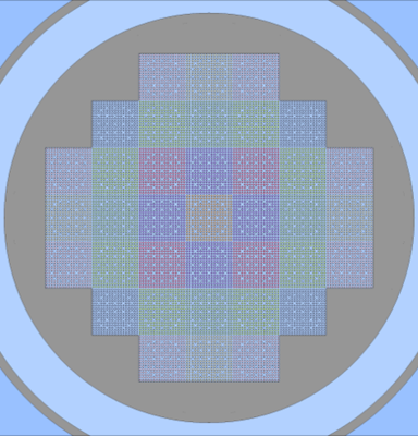
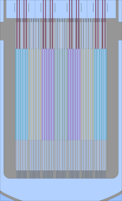
The modelled SMR is the same 37 assembly Er-UO2 fuelled core that has been previously used for the demonstration of the depletion capabilities of Kraken:
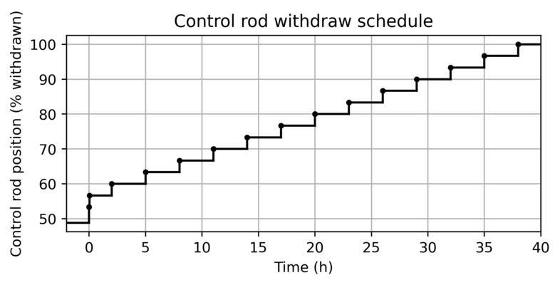
The transient starts from critical hot zero power (HZP) conditions (actually from 1 % power level) with all control rod banks at approximately 50 % insertion. The boron concentration in the coolant corresponds to the critical boron at all rods out (ARO) hot full power (HFP) conditions. The control rods are withdrawn from the core in a stepwise manner over 38 hours to allow for the accumulation of xenon in the core:
To reformulate the simulation setup:
- Evaluate (in a time-independent simulation) critical boron at hot full power all rods out conditions with convergence in
- Neutronics
- Thermal hydraulics
- Fuel temperature
- Xenon
- Using that critical boron, evaluate (in a time-independent simulation) critical control rod position at 1 % power level with convergence in
- Neutronics
- Thermal hydraulics
- Fuel temperature
- Xenon
- Save initial conditions from the 1 % power level time-independent calculation.
- Start a time dependent simulation from 1 % power level and slowly withdraw the control rods fully from the core.
If the time-independent and time-dependent calculation methodologies produce equivalent steady state solutions and have been correctly implemented, the simulation should (in the end) end up in the same state as the time-independent HFP ARO calculation.
Evaluating HFP ARO critical boron
The first part of the simulation is only needed here in order to obtain a more realistic and reasonable end state for the transient simulation by finding a realistic boron concentration for the coolant. The simulation is set up as a normal coupled steady state simulation between Ants and SUBCHANFLOW with Ants using its equilibrium xenon calculation mode and iterating the coolant boron concentration to reach a critical system. The system power is set to 50 MW, which corresponds to the nominal full power in the Er-UO2 core.
The Cerberus input used for the calculation is included below and is a rather simple coupled calculation input. It may be interesting to note that since Ants is developed in the Kraken context, many of the basic input data can be sent to Ants via Cerberus (control rod positions, system power, xenon calculation mode, iteration mode etc.). The same Ants input is actually used for all of the simulations here with the relevant parts of the Ants model being modified via Cerberus instead of in the Ants input file. Conversely, as SUBCHANFLOW is developed by KIT and the Kraken-coupling is achieved via a VTT written SUBCHANFLOW wrapper the amount of possible input data accessible via Cerberus is more limited and the steady state simulations use a (very slightly) different input file for SUBCHANFLOW than the transient simulation.
Cerberus input for HPF ARO boron iteration
from os import environ
from pathlib import Path

import numpy as np

import cerberus as cb
from cerberus.solvers import CodeInput
from cerberus.solvers import Solver
from cerberus.interpolation import Interpolator
from numpy.core.fromnumeric import size

# Verbosity for terminal output of Cerberus

cb.LOG.set_verbosity(1)

# Create and start solvers

solver_defs = [["SCF", environ["SCFWRAP_EXE_PATH"], [], ["../Inputs/scf/input_steady.txt"]],
               ["ANTS", environ["ANTS_EXE_PATH"], ["--cerberus","--port"], ["../Inputs/Ants.inp"]]]

solvers = {}

port_number = 2211

for name, solver_path, params, inputs in solver_defs:

    # Create input

    solver_input = CodeInput(name, inputs)

    # Create solver

    solver = Solver(name, solver_path, params)
    solver.input = solver_input
    solver.initialize(port_number)

    # Add to solver dict

    solvers[name] = solver

    port_number += 1

# Alias variables for solvers

scf = solvers["SCF"]
ants = solvers["ANTS"]

# Get SCF fields needed for coupled calculation

scf_cool_temperature = scf.get_transferrable("scf_of_cool_temperature_chan")
scf_cool_density = scf.get_transferrable("scf_of_cool_density_chan")
scf_fuel_temperature = scf.get_transferrable("scf_of_fuel_temperature_vol_ave")
scf_power = scf.get_transferrable("scf_if_fuel_power")

# Get Ants fields needed for coupled calculation

ants_cool_temperature = ants.get_transferrable("Ants_if_coolant_temperature")
ants_cool_density = ants.get_transferrable("Ants_if_coolant_density")
ants_fuel_temperature = ants.get_transferrable("Ants_if_fuel_temperature")
ants_power = ants.get_transferrable("Ants_of_supernode_power")
ants_boron = ants.get_transferrable("Ants_ov_boron")

# Create interpolators that handle data transfer between SCF and Ants

interp_ct = Interpolator.from_file(scf_cool_temperature,
                                   ants_cool_temperature,
                                   "../Inputs/scf_to_ants.txt")
interp_cd = Interpolator.from_file(scf_cool_density,
                                   ants_cool_density,
                                   "../Inputs/scf_to_ants.txt")
interp_ft = Interpolator.from_file(scf_fuel_temperature,
                                   ants_fuel_temperature,
                                   "../Inputs/scf_to_ants.txt")
interp_p = Interpolator.from_file(ants_power,
                                  scf_power,
                                  "../Inputs/ants_to_scf.txt")

################################################################################

# Setup some options for the Ants model

# 100 % power level (50 MW)

tra = ants.get_transferrable("Ants_iv_total_power")
tra.value_vec[0] = 50e6
tra.communicate()

# Equilibrium xenon (0 = zero, 1 = fixed, 2 = equilibrium, 3 = dynamic, 4 = depletion)

tra = ants.get_transferrable("Ants_iv_xenon_state")
tra.value_vec[0] = 2
tra.communicate()

# Control variable (iterate keff (1) or boron (2)?), here boron

tra = ants.get_transferrable("Ants_iv_control_variable")
tra.value_vec[0] = 2
tra.communicate()

# Initial value for keff

tra = ants.get_transferrable("Ants_iv_keff")
tra.value_vec[0] = 1.0
tra.communicate()

# Initial value for boron (ppm)

tra = ants.get_transferrable("Ants_iv_boron")
tra.value_vec[0] = 200.0
tra.communicate()

# Control rod position

height = 200.0

names = ["Ants_iv_cr_bank_height_CR2.1",
         "Ants_iv_cr_bank_height_CR2.2",
         "Ants_iv_cr_bank_height_CR2.3",
         "Ants_iv_cr_bank_height_CR2.4",
         "Ants_iv_cr_bank_height_CR4.1",
         "Ants_iv_cr_bank_height_CR4.2",
         "Ants_iv_cr_bank_height_CR4.3",
         "Ants_iv_cr_bank_height_CR4.4",
         "Ants_iv_cr_bank_height_CR6.1",
         "Ants_iv_cr_bank_height_CR6.2",
         "Ants_iv_cr_bank_height_CR6.3",
         "Ants_iv_cr_bank_height_CR6.4",
         "Ants_iv_cr_bank_height_CR6.5",
         "Ants_iv_cr_bank_height_CR6.6",
         "Ants_iv_cr_bank_height_CR6.7",
         "Ants_iv_cr_bank_height_CR6.8"]

for name in names:
    tra = ants.get_transferrable(name)
    tra.value_vec[0] = height
    tra.communicate()

################################################################################

# Initialize SCF power field (50 MW divided uniformly over SCF cells)

scf_power.value_vec = 50e6/scf_power.n_values*np.ones(scf_power.n_values)

################################################################################
################################################################################

# --- Coupled solution

max_iter = 50
for i in range(max_iter):
    # --- TH solution and communication

    scf_power.communicate()
    scf_power.write_simple(suffix_in=f"{i+1}")

    scf.solve()

    scf_cool_density.communicate()
    scf_cool_temperature.communicate()
    scf_fuel_temperature.communicate()

    # --- Transfers from SCF to Ants fields

    interp_ct.interpolate()
    interp_cd.interpolate()
    interp_ft.interpolate()

    # --- Neutronics solution and communication

    ants_cool_density.communicate()
    ants_cool_temperature.communicate()
    ants_fuel_temperature.communicate()

    ants.solve()

    ants_power.communicate()
    ants_boron.communicate()

    # --- Transfers from Ants to SCF

    interp_p.interpolate()

    print(f"Finished iteration {i+1}, boron is {ants_boron.value_vec[0]}")

# Choose field/value names to save
# (save HFP steady state fields so that we can compare our transient final state
#  to them)

to_save = ["Ants_ov_keff", "Ants_ov_boron",
           "Ants_if_fuel_temperature", "Ants_if_coolant_temperature",
           "Ants_if_coolant_density", "Ants_of_power",
           "Ants_of_number_density_xe135",
           "Ants_of_number_density_i135"]

# Output path. Create folder if necessary

output_path = Path(f"./output")
output_path.mkdir(exist_ok=True)
for name in to_save:
    tra = ants.get_transferrable(name)
    tra.communicate()
    tra.write_simple(suffix_in="final", folder_path=output_path)
As we can see from the Cerberus output, the coupled boron iteration convergences in a fast an orderly manner:
Part of Cerberus output for HPF ARO boron iteration
[...]
Finished iteration 1, boron is 228.22516244212167
Finished iteration 2, boron is 230.30442058656257
Finished iteration 3, boron is 183.30511926195726
Finished iteration 4, boron is 164.65050546550327
Finished iteration 5, boron is 157.30379476197407
Finished iteration 6, boron is 154.48212377902502
Finished iteration 7, boron is 153.39382413693164
Finished iteration 8, boron is 152.97112777866687
Finished iteration 9, boron is 152.8055417631042
Finished iteration 10, boron is 152.74065234508132
Finished iteration 11, boron is 152.71526006774332
Finished iteration 12, boron is 152.70531858406244
Finished iteration 13, boron is 152.70142257953808
Finished iteration 14, boron is 152.69989492714808
Finished iteration 15, boron is 152.69929592234286
Finished iteration 16, boron is 152.69906109695194
Finished iteration 17, boron is 152.69896905258145
Finished iteration 18, boron is 152.6989329754515
Finished iteration 19, boron is 152.6989188350551
Finished iteration 20, boron is 152.6989132928211
Finished iteration 21, boron is 152.69891112072364
Finished iteration 22, boron is 152.69891026952612
Finished iteration 23, boron is 152.69890993599222
Finished iteration 24, boron is 152.6989098053487
Finished iteration 25, boron is 152.69890975416695
Finished iteration 26, boron is 152.69890973416096
Finished iteration 27, boron is 152.69890972645177
Finished iteration 28, boron is 152.69890972349958
Finished iteration 29, boron is 152.69890972234265
Finished iteration 30, boron is 152.69890972197138
Finished iteration 31, boron is 152.69890972193002
Finished iteration 32, boron is 152.6989097219338
Finished iteration 33, boron is 152.69890972198456
Finished iteration 34, boron is 152.69890972208015
Finished iteration 35, boron is 152.69890972225545
Finished iteration 36, boron is 152.698909722428
Finished iteration 37, boron is 152.69890972246756
Finished iteration 38, boron is 152.69890972255268
Finished iteration 39, boron is 152.698909722585
Finished iteration 40, boron is 152.69890972268558
Finished iteration 41, boron is 152.6989097228531
Finished iteration 42, boron is 152.69890972296628
Finished iteration 43, boron is 152.69890972316364
Finished iteration 44, boron is 152.69890972327443
Finished iteration 45, boron is 152.69890972335577
Finished iteration 46, boron is 152.6989097234503
Finished iteration 47, boron is 152.69890972359548
Finished iteration 48, boron is 152.69890972363942
Finished iteration 49, boron is 152.69890972372042
Finished iteration 50, boron is 152.69890972382908
Evaluating critical control rod position at HZP fixed boron conditions
Cerberus input for HZP control rod iteration
Part of Cerberus output for HZP control rod iteration
[...]
Height is 150.0, keff is 1.0137994157229595 (based on 3 coupled iterations)
Height is 140.0, keff is 1.0097132150307848 (based on 3 coupled iterations)
Height is 130.0, keff is 1.004371680638068 (based on 3 coupled iterations)
Height is 120.0, keff is 0.9974297441040372 (based on 3 coupled iterations)
Height is 121.0, keff is 0.997992947986957 (based on 6 coupled iterations)
Height is 122.0, keff is 0.9986113787463294 (based on 6 coupled iterations)
Height is 123.0, keff is 0.999327881570897 (based on 6 coupled iterations)
Height is 124.0, keff is 1.000166398442108 (based on 6 coupled iterations)
Height is 123.9, keff is 1.0000762007919366 (based on 9 coupled iterations)
Height is 123.80000000000001, keff is 0.9999875162017355 (based on 9 coupled iterations)
Height is 123.81000000000002, keff is 0.9999963183709505 (based on 12 coupled iterations)
Height is 123.82000000000002, keff is 1.00000513516873 (based on 12 coupled iterations)
Height is 123.81900000000002, keff is 1.0000042528284148 (based on 15 coupled iterations)
Height is 123.81800000000001, keff is 1.000003370634821 (based on 15 coupled iterations)
Height is 123.81700000000001, keff is 1.0000024885879013 (based on 15 coupled iterations)
Height is 123.816, keff is 1.0000016066876227 (based on 15 coupled iterations)
Height is 123.815, keff is 1.0000007249339529 (based on 15 coupled iterations)
Height is 123.814, keff is 0.9999998433268541 (based on 15 coupled iterations)
Height is 123.8141, keff is 0.9999999314800674 (based on 18 coupled iterations)
Saving initial conditions for the transient
Cerberus input for the transient simulation


