SMR startup simulation (outdated)

Overview

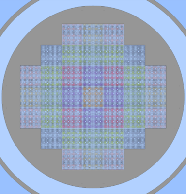
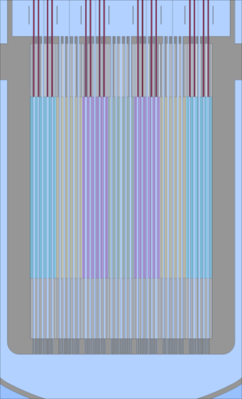
In order to test and demonstrate the time dependent calculation capabilities of the Kraken framework in a reasonably realistic context, a time dependent simulation was conducted of the initial rise to power of a small modular reactor (SMR) core. The simulation used the Ants nodal neutronics code to resolve the evolution of neutronics and the xenon fission poison chain in the system and the SUBCHANFLOW thermal hydraulics code to solve the coolant flow and heat transfer in fuel rods.

The modelled SMR is the same 37 assembly Er-UO₂ fuelled core that has been previously used for the demonstration of the depletion capabilities of Kraken:

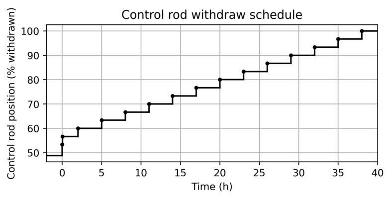
The transient starts from critical hot zero power (HZP) conditions (actually from 1 % power level) with all control rod banks at approximately 50 % insertion. The boron concentration in the coolant corresponds to the critical boron at all rods out (ARO) hot full power (HFP) conditions. The control rods are withdrawn from the core in a stepwise manner over 38 hours to allow for the accumulation of xenon in the core:

To reformulate the simulation setup:

• Evaluate (in a time-independent simulation) critical boron at hot full power all rods out conditions with convergence in
  • Neutronics
  • Thermal hydraulics
  • Fuel temperature
  • Xenon
• Using that critical boron, evaluate (in a time-independent simulation) critical control rod position at 1 % power level with convergence in
  • Neutronics
  • Thermal hydraulics
  • Fuel temperature
  • Xenon
• Save initial conditions from the 1 % power level time-independent calculation.
• Start a time dependent simulation from 1 % power level and slowly withdraw the control rods fully from the core.

If the time-independent and time-dependent calculation methodologies produce equivalent steady state solutions and have been correctly implemented, the simulation should (in the end) end up in the same state as the time-independent HFP ARO calculation.

Evaluating HFP ARO critical boron

The first part of the simulation is only needed here in order to obtain a more realistic and reasonable end state for the transient simulation by finding a realistic boron concentration for the coolant.

Cerberus input for HPF ARO boron iteration

from os import environ
from pathlib import Path

import numpy as np

import cerberus as cb
from cerberus.solvers import CodeInput
from cerberus.solvers import Solver
from cerberus.interpolation import Interpolator
from numpy.core.fromnumeric import size

# Verbosity for terminal output of Cerberus

cb.LOG.set_verbosity(1)

# Create and start solvers

solver_defs = [["SCF", environ["SCFWRAP_EXE_PATH"], [], ["./Inputs/scf/input.txt"]],
               ["ANTS", environ["ANTS_EXE_PATH"], ["--cerberus","--port"], ["./Inputs/Ants8g.inp"]]]

solvers = {}

port_number = 2211

for name, solver_path, params, inputs in solver_defs:

    # Create input

    solver_input = CodeInput(name, inputs)

    # Create solver

    solver = Solver(name, solver_path, params)
    solver.input = solver_input
    solver.initialize(port_number)

    # Add to solver dict

    solvers[name] = solver

    port_number += 1

# Alias variables for solvers

scf = solvers["SCF"]
ants = solvers["ANTS"]

# Get SCF fields needed for coupled calculation

scf_cool_temperature = scf.get_transferrable("scf_of_cool_temperature_chan")
scf_cool_density = scf.get_transferrable("scf_of_cool_density_chan")
scf_fuel_temperature = scf.get_transferrable("scf_of_fuel_temperature_vol_ave")
scf_power = scf.get_transferrable("scf_if_fuel_power")

# Initialize SCF power field (50 MW divided uniformly over SCF cells)

scf_power.value_vec = 50e6/scf_power.n_values*np.ones(scf_power.n_values)

# Get Ants fields needed for coupled calculation

ants_cool_temperature = ants.get_transferrable("Ants_if_coolant_temperature")
ants_cool_density = ants.get_transferrable("Ants_if_coolant_density")
ants_fuel_temperature = ants.get_transferrable("Ants_if_fuel_temperature")
ants_power = ants.get_transferrable("Ants_of_supernode_power")
ants_boron = ants.get_transferrable("Ants_ov_boron")

# Create interpolators that handle data transfer between SCF and Ants

interp_ct = Interpolator.from_file(scf_cool_temperature,
                                   ants_cool_temperature,
                                   "./Inputs/scf_to_ants.txt")
interp_cd = Interpolator.from_file(scf_cool_density,
                                   ants_cool_density,
                                   "./Inputs/scf_to_ants.txt")
interp_ft = Interpolator.from_file(scf_fuel_temperature,
                                   ants_fuel_temperature,
                                   "./Inputs/scf_to_ants.txt")
interp_p = Interpolator.from_file(ants_power,
                                  scf_power,
                                  "./Inputs/ants_to_scf.txt")


################################################################################
################################################################################

# --- Coupled solution

max_iter = 50
for i in range(max_iter):
    # --- TH solution and communication

    scf_power.communicate()
    scf_power.write_simple(suffix_in=f"{i+1}")

    scf.solve()

    scf_cool_density.communicate()
    scf_cool_temperature.communicate()
    scf_fuel_temperature.communicate()

    # --- Transfers from SCF to Ants fields

    interp_ct.interpolate()
    interp_cd.interpolate()
    interp_ft.interpolate()

    # --- Neutronics solution and communication

    ants_cool_density.communicate()
    ants_cool_temperature.communicate()
    ants_fuel_temperature.communicate()

    ants.solve()

    ants_power.communicate()
    ants_boron.communicate()

    # --- Transfers from Ants to SCF

    interp_p.interpolate()

    print(f"Finished iteration {i+1}, boron is {ants_boron.value_vec[0]}")

# Choose field/value names to save

to_save = ["Ants_ov_keff", "Ants_ov_boron"]

# Output path. Create folder if necessary

output_path = Path(f"./output")
output_path.mkdir(exist_ok=True)
for name in to_save:
    tra = ants.get_transferrable(name)
    tra.communicate()
    tra.write_simple(suffix_in="final", folder_path=output_path)

As we can see from the Cerberus output, the coupled boron iteration convergences in a fast an orderly manner:

Part of Cerberus output for HPF ARO boron iteration

[...]
Finished iteration 1, boron is 241.11834260327765
Finished iteration 2, boron is 215.2718468141726
Finished iteration 3, boron is 185.87313896299054
Finished iteration 4, boron is 173.3774955250355
Finished iteration 5, boron is 168.31982440765557
Finished iteration 6, boron is 166.3256614351459
Finished iteration 7, boron is 165.53688601838087
Finished iteration 8, boron is 165.22148909036616
Finished iteration 9, boron is 165.09469219902923
Finished iteration 10, boron is 165.04377146267225
Finished iteration 11, boron is 165.02336734511402
Finished iteration 12, boron is 165.01519526343998
Finished iteration 13, boron is 165.01192023059554
Finished iteration 14, boron is 165.0106071995804
Finished iteration 15, boron is 165.01008083684778
Finished iteration 16, boron is 165.009869886424
Finished iteration 17, boron is 165.00978535429869
Finished iteration 18, boron is 165.00975148002664
Finished iteration 19, boron is 165.00973790527965
Finished iteration 20, boron is 165.00973246550984
Finished iteration 21, boron is 165.00973028562225
Finished iteration 22, boron is 165.00972941228162
Finished iteration 23, boron is 165.0097290626322
Finished iteration 24, boron is 165.0097289227151
Finished iteration 25, boron is 165.00972886671116
Finished iteration 26, boron is 165.00972884451494
Finished iteration 27, boron is 165.0097288358948
Finished iteration 28, boron is 165.00972883263654
Finished iteration 29, boron is 165.00972883156635
Finished iteration 30, boron is 165.00972883135597
Finished iteration 31, boron is 165.0097288315159
Finished iteration 32, boron is 165.00972883175677
Finished iteration 33, boron is 165.00972883202363
Finished iteration 34, boron is 165.0097288323592
Finished iteration 35, boron is 165.00972883264916
Finished iteration 36, boron is 165.00972883298
Finished iteration 37, boron is 165.00972883338346
Finished iteration 38, boron is 165.0097288337177
Finished iteration 39, boron is 165.00972883415443
Finished iteration 40, boron is 165.00972883451635
Finished iteration 41, boron is 165.00972883482027
Finished iteration 42, boron is 165.00972883515766
Finished iteration 43, boron is 165.00972883553914
Finished iteration 44, boron is 165.00972883589347
Finished iteration 45, boron is 165.00972883625684
Finished iteration 46, boron is 165.00972883659034
Finished iteration 47, boron is 165.00972883682405
Finished iteration 48, boron is 165.00972883721238
Finished iteration 49, boron is 165.00972883759266
Finished iteration 50, boron is 165.00972883793503