Difference between revisions of "Kharon input manual"

Revision as of 14:09, 6 June 2019

The Kharon input is a keyword input. It consists of several grouped input parameters. Each group starts with the keyword that defines the group (name of the group), possibly followed by data entries associated with the keyword. The group can consist of several keyword (parameter name) and value pairs that are enclosed within a set of curly brackets.

A working input file consists of several input groups.

The order of the groups or the parameter name and value pairs within the group is not important.

The input file can contain comments: all characters after '#', '!', and '%' on each line are considered as comments.

All keywords, operators, and data entries must be separated by one or more spaces or line changes, since they are regarded as words.

Input groups

Apart from the assembly numbering, at the end, all of the following input groups are required for a working input file. To distinguish between mandatory and optional parameters, the mandatory parameters are colored in red and the optional parameters in green.

Simulation control parameters

The keyword that defines this group is simulationControl. As the name suggests, these parameters are used to control the solution flow. The bare minimum is to provide a value for the number of phases, nPhases.

Keyword	Size and type	Valid options / Valid range	Default	Description
nPhases	1*integer	1 = single-phase water or 2 = water and steam		Number of phases.
nIterMax	1*integer	positive integer	500	Number of solution (outer) iterations.
urfU	1*real	[0, 1]	0.5	Under-relaxation factor for velocity [-].
urfP	1*real	[0, 1]	0.5	Under-relaxation factor for pressure [-].
urfH	1*real	[0, 1]	0.9	Under-relaxation factor for enthalpy [-].
gravity	1*real	( $-\infty$ , $\infty$ )	-9.81	Gravitational acceleration (in the direction of positive z-coordinate; upwards) [m/s²]
readRestart	1*integer	0 = No, 1 = Yes	0	Start from a previously saved state?
standAlone	1*integer	0 = Multiphysics coupling, 1 = Stand-alone simulation	0	Start a stand-alone simulation?
writeFormat	1*word	ascii, binary	ascii	Write format for output fields
materialProperties	1*word	libTable, libFluid	libTable	Calculation of material properties: libTable = linear interpolation from a pretabulated set of material properties, libFluid = IAPWS standard polynomial functions.
thermalBC	1*word	power, heatFlux, wallTemperature	heatFlux	Thermal boundary condition: power = set the power to each cell (Kharon converts this to heat flux and calculates the surface temperature distribution), heatFlux = set the heat flux of the heated surfaces in each cell (Kharon converts this to power and calculates the surface temperature distribution), wallTemperature = set the surface temperature of the heated surfaces in each cell (Kharon calculates the heat flux and power distributions).

An example with the simulation control default values for a single-phase case is:

simulationControl
{
    nPhases            1
    nIterMax           500
    urfU               0.5
    urfP               0.5
    urfH               0.9
    gravity            -9.81
    readRestart        0
    standAlone         0
    writeFormat        ascii
    materialProperties libTable
    thermalBC          heatFlux
}

Inlet definition

The keyword that defines this group is inlet. There are four available inlet types to choose from: pressureInlet, velocityInlet, massFlowInlet, totalMassFlowInlet. The inlet type determines the parameter that is required to define the flow into the domain.

Pressure inlet

Keyword	Size and type	Valid options / Valid range	Description
type	1*word	pressureInlet	Defines a pressure inlet.
pressure	1*real	[0, $\infty$ )	Absolute (static) pressure at inlet [Pa].

Velocity inlet

Keyword	Size and type	Valid options / Valid range	Description
type	1*word	velocityInlet	Defines a velocity inlet.
velocity	nPhases*real	[0, $\infty$ )	Phase velocities at inlet [m/s].

Mass flow inlet

Keyword	Size and type	Valid options / Valid range	Description
type	1*word	massFlowInlet	Defines a mass flow inlet.
massFlowRate	nPhases*real	[0, $\infty$ )	Phase mass flow rates per assembly [kg/s].

Total mass flow inlet

Keyword	Size and type	Valid options / Valid range	Description
type	1*word	totalMassFlowInlet	Defines a total mass flow inlet.
massFlowRate	1*real	[0, $\infty$ )	Total mass flow rate into the core [kg/s].

Common inlet parameters

In addition to the inlet type specific parameters shown above, the following parameters need to be given for all inlet types:

Keyword	Size and type	Valid options / Valid range	Description
temperature	nPhases*real	[0, $\infty$ )	Phase temperatures at inlet [K].
volumeFraction	nPhases*real	[0, 1]	Phase volume fractions at inlet [-].

An example of a mass flow inlet for a single-phase simulation is given below:

inlet
{
    type               massFlowInlet
    massFlowRate       116.56            ! [kg/s] per assembly
    temperature        562.0             ! [K]
    volumeFraction     1.0               ! [-]
}

The same exact boundary condition for a two-phase simulation is:

inlet
{
    type               massFlowInlet
    massFlowRate       116.56    0.0     ! [kg/s] per assembly
    temperature        562.0     618.97  ! [K]
    volumeFraction     1.0       0.0     ! [-]
}

Outlet definition

The keyword that defines this group is outlet. The following parameters need to be provided:

Keyword	Size and type	Valid options / Valid range	Description
pressure	1*real	[0, $\infty$ )	Absolute (static) pressure at outlet [Pa].
temperature	nPhases*real	[0, $\infty$ )	Phase temperatures at outlet (for backflow) [K].
volumeFraction	nPhases*real	[0, 1]	Phase volume fractions at outlet (for backflow) [-].

An example of an outlet definition for a single-phase simulation is given below:

outlet
{
    pressure           15.7e6            ! [Pa]
    temperature        618.97            ! [K]
    volumeFraction     1.0               ! [-]
}

The same exact definition for a two-phase simulation is:

outlet
{
    pressure           15.7e6            ! [Pa]
    temperature        618.97    618.97  ! [K]
    volumeFraction     1.0       0.0     ! [-]
}

List of fuel types

The keyword that defines this group is fuelType, which is immediately followed by the fuel type name. Several different fuel types can be defined, which can then referred to by its name when defining the core load pattern.

Keyword	Size and type	Valid options / Valid range	Default	Description
nCells	1*integer	[1, $\infty$ )		Number of cells along the height of the fuel assembly.
nPins	1*integer	[1, $\infty$ )	1	Number of fuel pins for heat transfer / temperature solution.
bottomElevation	1*real	( $-\infty$ , $\infty$ )		Elevation of the assembly inlet (z-coordinate) [m]. Used for post-processing.
cellHeight	nCells*real	(0, $\infty$ )		Cell height [m].
hydraulicDiameter	nCells*real	(0, $\infty$ )		Hydraulic diameter [m].
thermalDiameter	nPinsnCellsreal	(0, $\infty$ )		Thermal diameter [m].
porosity	nCells*real	(0, 1]		Porosity, fluid fraction of total volume [m].

Two operators, * and x, are available to abbreviate the notation when setting the porosities and diameters, in particular.

An integer value times (*) a real value is replaced in its place with the number of said real values. A combination of separate real values and real values given with the *-operator can be used as well. This way you can provide the values for cell height, porosity of the assembly, hydraulic diameter of the assembly, and thermal diameter of a single pin, e.g. porosity of an assembly consisting of 21 cells can be given by: 10 * 0.5 0.5 10 * 0.5 = 0.5 10 * 0.5 10 * 0.5 = 21 * 0.5.

To facilitate definition of the thermal diameters for multiple pin assemblies, the x-operator is introduced. You first need to define the thermal diameters for a single pin. Multiple copies of that pin can be created with the x-operator: 3 x 21 * 0.01 = 21 * 0.01 21 * 0.01 21 * 0.01. Note that you need to use spaces around the x-operator, since otherwise it will be confused as a word.

In the following two identical fuel types, f1 and f2, are defined using a different number of pins for the heat transfer / temperature solution:

fuelType f1
{
    nCells             20
    bottomElevation    0.0
    cellHeight         20 * 0.1
    hydraulicDiameter  20 * 0.0110946
    thermalDiameter    20 * 0.0124111
    porosity           20 * 0.530672
}

fuelType f2
{
    nCells             20
    nPins              265
    bottomElevation    0.0
    cellHeight         20 * 0.1
    hydraulicDiameter  20 * 0.0110946
    thermalDiameter    265 x 20 * 3.28893
    porosity           20 * 0.530672
}

Core definition

The keyword that defines this group is core. This group sets the geometry of the core, namely the core lattice (square or hexagonal) and assembly pitch.

Keyword	Size and type	Valid options / Valid range	Description
coreLattice	1*word	square, hexagonal	Core lattice.
assemblyPitch	1*real	(0, $\infty$ )	Assembly pitch [m].

An example of a core definition with a square lattice is given below:

core
{
    coreLattice        square
    assemblyPitch      0.2150364
}

An example of hexagonal core definition is:

core
{
    coreLattice        hexagonal
    assemblyPitch      0.236
}

Load pattern

The keyword that defines this group is loadPattern. Together with the core definition above, the geometry of the core is fully defined. The output mesh can be generated based on these two input groups. The load pattern consists of the fuel type names defined above that basically provide a map of the core. Empty locations are denoted by zeros. An example of an EPR-like core is given below. Since the core and loadPattern groups are closely linked, it is good practice to give them together in the input file.

core
{
    coreLattice        square
    assemblyPitch      0.2150364
}

loadPattern
{
        0    0    0    0    0   f2   f2   f2   f2   f2    0    0    0    0    0
        0    0    0   f2   f2   f2   f1   f1   f1   f2   f2   f2    0    0    0
        0    0   f2   f2   f1   f1   f1   f1   f1   f1   f1   f2   f2    0    0
        0   f2   f2   f1   f1   f1   f1   f1   f1   f1   f1   f1   f2   f2    0
        0   f2   f1   f1   f1   f1   f1   f1   f1   f1   f1   f1   f1   f2    0
       f2   f2   f1   f1   f1   f1   f1   f1   f1   f1   f1   f1   f1   f2   f2
       f2   f1   f1   f1   f1   f1   f1   f1   f1   f1   f1   f1   f1   f1   f2
       f2   f1   f1   f1   f1   f1   f1   f1   f1   f1   f1   f1   f1   f1   f2
       f2   f1   f1   f1   f1   f1   f1   f1   f1   f1   f1   f1   f1   f1   f2
       f2   f2   f1   f1   f1   f1   f1   f1   f1   f1   f1   f1   f1   f2   f2
        0   f2   f1   f1   f1   f1   f1   f1   f1   f1   f1   f1   f1   f2    0
        0   f2   f2   f1   f1   f1   f1   f1   f1   f1   f1   f1   f2   f2    0
        0    0   f2   f2   f1   f1   f1   f1   f1   f1   f1   f2   f2    0    0
        0    0    0   f2   f2   f2   f1   f1   f1   f2   f2   f2    0    0    0
        0    0    0    0    0   f2   f2   f2   f2   f2    0    0    0    0    0
}

An example of a hexagonal core (VVER-1000) is given below. The array is tilted to produce a better visualization of the core.

core
{
    coreLattice        hexagonal
    assemblyPitch      0.236
}

loadPattern
{
        0     0     0     0     0     0     0     0    f1    f1    f1    f1    f1    f1     0

           0     0     0     0     0     0    f1    f1    f1    f1    f1    f1    f1    f1    f1

              0     0     0     0     0    f1    f1    f1    f1    f1    f1    f1    f1    f1    f1 

                 0     0     0     0    f1    f1    f1    f1    f1    f1    f1    f1    f1    f1    f1 

                    0     0     0    f1    f1    f1    f1    f1    f1    f1    f1    f1    f1    f1    f1 

                       0     0    f1    f1    f1    f1    f1    f1    f1    f1    f1    f1    f1    f1    f1

                          0    f1    f1    f1    f1    f1    f1    f1    f1    f1    f1    f1    f1    f1    f1

                             0    f1    f1    f1    f1    f1    f1    f1    f1    f1    f1    f1    f1    f1     0

                               f1    f1    f1    f1    f1    f1    f1    f1    f1    f1    f1    f1    f1    f1     0

                                  f1    f1    f1    f1    f1    f1    f1    f1    f1    f1    f1    f1    f1     0     0

                                     f1    f1    f1    f1    f1    f1    f1    f1    f1    f1    f1    f1     0     0     0

                                        f1    f1    f1    f1    f1    f1    f1    f1    f1    f1    f1     0     0     0     0

                                           f1    f1    f1    f1    f1    f1    f1    f1    f1    f1     0     0     0     0     0

                                              f1    f1    f1    f1    f1    f1    f1    f1    f1     0     0     0     0     0     0

                                                  0    f1    f1    f1    f1    f1    f1     0     0     0     0     0     0     0     0
}

Assembly numbering (optional)

The keyword that defines this group is assemblyNumbering. This allows to set an arbitrary numbering for the assemblies. The pattern should be identical in shape and size to loadPattern. The default numbering should not be changed when running coupled multiphysics simulations, since it will mess up the field coupling in Cerberus! The following produces the default assembly numbering for the hexagonal core above:

assemblyNumbering
{
        0     0     0     0     0     0     0     0     1     2     3     4     5     6     0

           0     0     0     0     0     0     7     8     9    10    11    12    13    14    15

              0     0     0     0     0    16    17    18    19    20    21    22    23    24    25

                 0     0     0     0    26    27    28    29    30    31    32    33    34    35    36

                    0     0     0    37    38    39    40    41    42    43    44    45    46    47    48

                       0     0    49    50    51    52    53    54    55    56    57    58    59    60    61

                          0    62    63    64    65    66    67    68    69    70    71    72    73    74    75

                             0    76    77    78    79    80    81    82    83    84    85    86    87    88     0

                               89    90    91    92    93    94    95    96    97    98    99   100   101   102     0

                                 103   104   105   106   107   108   109   110   111   112   113   114   115     0     0

                                   116    117   118   119   120   121   122   123   124   125   126   127     0     0     0

                                      128    129   130   131   132   133   134   135   136   137   138     0     0     0     0

                                          139   140   141   142   143   144   145   146   147   148     0     0     0     0     0

                                             149   150   151   152   153   154   155   156   157     0     0     0     0     0     0

                                                  0   158   159   160   161   162   163     0     0     0     0     0     0     0     0
}

Geometric input parameters

Figure 1: Cross section of an EPR fuel assembly.

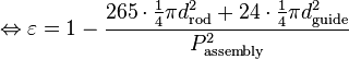
Porosity, $\varepsilon$ [-], is defined as the fluid fraction of total volume, which for a 1D channel is equivalent to the ratio of surface areas. Porosity of an EPR fuel assembly cross-section, shown in Figure 1, can be calculated from:

$\varepsilon = \frac{A_{\text{fluid}}}{A_{\text{assembly}}} = \frac{A_{\text{assembly}} - A_{\text{rod}} - A_{\text{guide}}} {A_{\text{assembly}}} = 1 - \frac{A_{\text{rod}} + A_{\text{guide}}}{A_{\text{assembly}}}$

(1)

$\Leftrightarrow \varepsilon = 1 - \frac{265 \cdot \tfrac{1}{4} \pi d^2_{\text{rod}} + 24 \cdot \tfrac{1}{4} \pi d^2_{\text{guide}}} {P^2_{\text{assembly}}}$

(2)

$\Leftrightarrow \varepsilon = 1 - \frac{265 \cdot \tfrac{1}{4} \pi \left( 0.0094996 \, \text{m}\right)^2 + 24 \cdot \tfrac{1}{4} \pi \left( 0.012446 \, \text{m}\right)^2} {\left( 0.2150364 \, \text{m}\right)^2} \approx 0.530672$

(3)

where:

$A_{\text{assembly}}$	cross-sectional area of the assembly [m²],
$A_{\text{fluid}}$	cross-sectional area available for fluid flow [m²],
$A_{\text{guide}}$	cross-sectional area of control rod guide tubes [m²],
$A_{\text{rod}}$	cross-sectional area of fuel rods [m²],
$d_{\text{guide}}$	control rod guide tube outer diameter [m],
$d_{\text{rod}}$	fuel rod outer diameter [m] and
$P_{\text{assembly}}$	assembly pitch [m].

Hydraulic diameter for the cross-section in Figure 1 can be calculated from:

$D_{\text{h}} = \frac{4 A_{\text{f}}}{P_{\text{w}}} = \frac{4 \varepsilon A_{\text{assembly}}} {P_{\text{w}}} = \frac{4 \varepsilon P^2_{\text{assembly}}} {265 \cdot \pi d_{\text{rod}} + 24 \cdot \pi d_{\text{guide}}} = \frac{4 \cdot 0.530672 \cdot \left( 0.2150364 \, \text{m}\right)^2} {265 \cdot \pi \cdot 0.0094996 \, \text{m} + 24 \cdot \pi \cdot 0.012446 \, \text{m}} \approx 0.0110946 \, \text{m}$

(4)

If the boundary conditions are provided for the average pin, i.e. power is averaged over the fuel assembly cross-section in Figure 1, the thermal diameter is calculated from:

$D_{\text{t}} = \frac{4 A_{\text{f}}}{P_{\text{h}}} = \frac{4 \varepsilon A_{\text{assembly}}} {P_{\text{t}}} = \frac{4 \varepsilon P^2_{\text{assembly}}} {265 \cdot \pi d_{\text{rod}}} = \frac{4 \cdot 0.530672 \cdot \left( 0.2150364 \, \text{m}\right)^2} {265 \cdot \pi \cdot 0.0094996 \, \text{m}} \approx 0.0124111 \, \text{m}$

(5)

where:

$D_{\text{h}}$	hydraulic diameter [m],
$D_{\text{t}}$	thermal diameter [m],
$P_{\text{h}}$	heated perimeter [m] and
$P_{\text{w}}$	wetted perimeter [m].

@@ Line 16: / Line 16: @@
 === Simulation control parameters ===
-The keyword that defines this group is '''simulationControl'''. The following parameters can be set inside this group. The bare minimum is to provide a value for the number of phases, ''nPhases''.
+The keyword that defines this group is '''simulationControl'''. As the name suggests, these parameters are used to control the solution flow. The bare minimum is to provide a value for the number of phases, ''nPhases''.
 {|class="wikitable" style="text-align: left;"

Difference between revisions of "Kharon input manual"

Revision as of 14:09, 6 June 2019

Contents

Input groups

Simulation control parameters

Inlet definition

Pressure inlet

Velocity inlet

Mass flow inlet

Total mass flow inlet

Common inlet parameters

Outlet definition

List of fuel types

Core definition

Load pattern

Assembly numbering (optional)

Geometric input parameters

Navigation menu

Personal tools

Namespaces

Variants

Views

More

Search

Navigation

Tools