Difference between revisions of "Mesh types"
(→Type 9 — List) |
|||
| Line 379: | Line 379: | ||
| '''10''' | | '''10''' | ||
| Number of values in the list. | | Number of values in the list. | ||
| + | |} | ||
| + | |||
| + | === Type 10 — Mixed nested mesh <span id="mixed nested mesh"></span>=== | ||
| + | |||
| + | The mixed nested mesh consists of a top level mesh (of any other mesh type) whose each cell may be filled with a sub-mesh of any kind. | ||
| + | |||
| + | {|class="wikitable" style="text-align: left;" | ||
| + | ! Data type/size | ||
| + | ! Data content (explanation) | ||
| + | ! Data content (example) | ||
| + | ! Notes | ||
| + | |- | ||
| + | | 1*integer | ||
| + | | Mesh type | ||
| + | | '''10''' | ||
| + | | | ||
| + | |- | ||
| + | | 1*integer | ||
| + | | Top mesh type | ||
| + | | '''1''' | ||
| + | | Would be structured regular Cartesian. | ||
| + | |- | ||
| + | | data type and size is dependent on top mesh type | ||
| + | | ... ''The rest of the top mesh data.'' | ||
| + | | '''2 2 1 -20.0 20.0 -20.0 20.0 -100.0 100.0''' | ||
| + | | Would be a 2x2x1 Cartesian mesh. | ||
| + | |- | ||
| + | | | ||
| + | | | ||
| + | | | ||
| + | | | ||
| + | |- | ||
| + | | 1*integer | ||
| + | | N<sub>m</sub> | ||
| + | | '''3''' | ||
| + | | Number of different sub-meshes in top mesh cells. | ||
| + | |- | ||
| + | | | ||
| + | | ''Information on'' N<sub>m</sub> ''sub-meshes'' | ||
| + | | | ||
| + | | | ||
| + | |- | ||
| + | | | ||
| + | | | ||
| + | | | ||
| + | | | ||
| + | |- | ||
| + | | 1*integer | ||
| + | | Sub-mesh 1 type | ||
| + | | '''1''' | ||
| + | | Would be structured regular Cartesian. | ||
| + | |- | ||
| + | | data type and size is dependent on sub-mesh type | ||
| + | | ''The rest of the sub-mesh 1 data.'' | ||
| + | | '''2 2 1 -10.0 10.0 -10.0 10.0 -100.0 100.0''' | ||
| + | | Would be a 2x2x1 Cartesian mesh. | ||
| + | |- | ||
| + | | | ||
| + | | | ||
| + | | | ||
| + | | | ||
| + | |- | ||
| + | | 1*integer | ||
| + | | Sub-mesh 2 type | ||
| + | | '''1''' | ||
| + | | Would be structured regular Cartesian. | ||
| + | |- | ||
| + | | data type and size is dependent on sub-mesh type | ||
| + | | ''The rest of the mesh 2 data.'' | ||
| + | | '''1 1 1 -10.0 10.0 -10.0 10.0 -100.0 100.0''' | ||
| + | | Would be a 1x1x1 Cartesian mesh. | ||
| + | |- | ||
| + | | | ||
| + | | | ||
| + | | | ||
| + | | | ||
| + | |- | ||
| + | | 1*integer | ||
| + | | Mesh N<sub>m</sub> type (lowest level) | ||
| + | | '''1''' | ||
| + | | Would be structured regular Cartesian. | ||
| + | |- | ||
| + | | data type and size is dependent on sub-mesh type | ||
| + | | ''The rest of the sub-mesh'' N<sub>m</sub> ''data.'' | ||
| + | | '''3 3 1 -10.0 10.0 -10.0 10.0 -100.0 100.0''' | ||
| + | | Would be a 3x3x3 Cartesian mesh. | ||
| + | |- | ||
| + | | | ||
| + | | | ||
| + | | | ||
| + | | | ||
| + | |- | ||
| + | | N<sup>top</sup><sub>c</sub>*integer | ||
| + | | Index of sub-mesh in each cell of the top mesh. | ||
| + | | ''' 1 2 1 3''' | ||
| + | | N<sup>top</sup><sub>c</sub> is the number of cells in the top mesh | ||
|} | |} | ||
Revision as of 20:45, 14 August 2023
Contents
Mesh types
Each physical data field consists of values on a specific mesh. Whereas several mesh types should be supported by Cerberus, the individual solvers typically only need to support their own mesh types. This section describes the geometry of the different mesh types supported by Cerberus and the mesh-data (the ordered list of values exactly specifying the mesh) associated with each mesh type.
Type 1 — Structured regular Cartesian mesh
Structured regular Cartesian meshes (in Kraken) are 3D meshes that cover a cuboid volume ([xmin, xmax]*[ymin, ymax]*[zmin, zmax]) and have a fixed number of cells in the x-, y- and z-direction (Nx, Ny, Nz). The total number of cells is the product of the number of cells in each of the three coordinate directions. The size/spacing of the cells is constant, but can be different for the different directions.
The mesh data for structured Cartesian meshes is as follows
| Data type/size | Data content (explanation) | Data content (example) | Notes |
|---|---|---|---|
| 1*integer | Mesh type | 1 | |
| Information on mesh size | |||
| 1*integer | Nx | 2 | Number of cells in X-direction. |
| 1*integer | Ny | 1 | Number of cells in Y-direction. |
| 1*integer | Nz | 4 | Number of cells in Z-direction. |
| Information on mesh boundaries | |||
| 2*float | xmin, xmax | -10.0, 10.0 | The outer limits of the mesh. |
| 2*float | ymin, ymax | -5.0, 5.0 | The outer limits of the mesh. |
| 2*float | zmin, zmax | 0.0, 100.0 | The outer limits of the mesh. |
Default indexing
x runs fastest, then y and finally z slowest.
All indices increase from minimum coordinate to maximum coordinate.
Type 2 — Structured irregular Cartesian mesh
Structured Cartesian meshes (in Kraken) are 3D meshes that cover a cuboid volume ([xmin, xmax]*[ymin, ymax]*[zmin, zmax]) and have a fixed number of cells in the x-, y- and z-direction (Nx, Ny, Nz). The total number of cells is the product of the number of cells in each of the three coordinate directions. For the irregular version, the size/spacing of the cells need not be constant.
The mesh data for structured irregular Cartesian meshes is as follows
| Data type/size | Data content (explanation) | Data content (example) | Notes |
|---|---|---|---|
| 1*integer | Mesh type | 2 | |
| Information on mesh size | |||
| 1*integer | Nx | 2 | Number of cells in X-direction. |
| 1*integer | Ny | 1 | Number of cells in Y-direction. |
| 1*integer | Nz | 4 | Number of cells in Z-direction. |
| Information on mesh boundaries | |||
| (Nx+1)*float | x0, x1, ..., xNx+1 | -10.0, -5.0, 10.0 | The cell boundaries in X-direction. |
| (Ny+1)*float | y0, y1, ..., yNy+1 | -5.0, 5.0 | The cell boundaries in Y-direction. |
| (Nz+1)*float | z0, z1, ..., zNz+1 | 0.0, 35.0, 50.0, 65.0, 100.0 | The cell boundaries in Z-direction. |
Default indexing
x runs fastest, then y and finally z slowest.
All indices increase from minimum coordinate to maximum coordinate.
Types 3-6 — Structured hexagonal meshes
Four different hexagonal meshes are currently supported (types 3-6). The different mesh types correspond to different orientations of the hexagons and to different choices of basis vectors.
The mesh data for all structured hexagonal meshes is the same:
| Data type/size | Data content (explanation) | Data content (example) | Notes |
|---|---|---|---|
| 1*integer | Mesh type | 3 | |
| Information on mesh size | |||
| 1*integer | Nx | 4 | Number of cells in X-direction. |
| 1*integer | Ny | 4 | Number of cells in Y-direction. |
| 1*integer | Nz | 4 | Number of cells in Z-direction. |
| Information on horizontal mesh geometry | |||
| 2*float | x0, y0 | 0.0, 0.0 | The horizontal centerpoint of the mesh. |
| 1*float | pitch | 0.236 | The horizontal pitch between adjacent mesh cells. |
| Information on axial boundaries | |||
| (Nz+1)*float | z0, z1, ..., zNz+1 | 0.0, 0.35, 0.50, 0.65, 1.0 | The cell boundaries in Z-direction. |
The following subsections show the base indexing in the different mesh types.
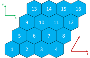
Type 3 — Structured x-type 60 degree hexagonal mesh
A single axial layer of the x-type (pointy top) hexagonal mesh with a 60 degree angle between the basis vectors is shown here:
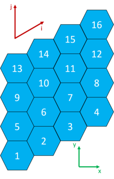
Type 4 — Structured y-type 60 degree hexagonal mesh
A single axial layer of the y-type (flat top) hexagonal mesh with a 60 degree angle between the basis vectors is shown here:
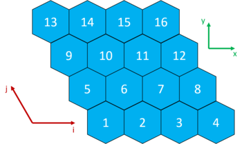
Type 5 — Structured x-type 120 degree hexagonal mesh
A single axial layer of the x-type (pointy top) hexagonal mesh with a 120 degree angle between the basis vectors is shown here:
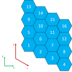
Type 6 — Structured y-type 120 degree hexagonal mesh
A single axial layer of the y-type (flat top) hexagonal mesh with a 120 degree angle between the basis vectors is shown here:
Type 7 — Structured cylindrical mesh
The mesh data for structured cylindrical meshes is as follows
| Data type/size | Data content (explanation) | Data content (example) | Notes |
|---|---|---|---|
| 1*integer | Mesh type | 7 | |
| Information on mesh size | |||
| 1*integer | Nr | 5 | Number of radial cells. |
| 1*integer | Nphi | 1 | Number of angular cells. |
| Information on mesh boundaries | |||
| (Nr + 1)*float | r0, r1, r2, ... | 0.0, 0.1e-2, 0.2e-2, 0.3e-2, 0.4e-2 | The cell boundaries for the mesh in the radial direction. |
| (Nphi + 1)*float | phi0, phi1, phi2, ... | 0, 360 | The cell boundaries for the mesh in the angular direction (degrees, as in polar coordinates). |
Default indexing
Radial indexing runs fastest and angular indexing slower.
Type 8 — Nested mesh
| Data type/size | Data content (explanation) | Data content (example) | Notes |
|---|---|---|---|
| 1*integer | Mesh type | 8 | |
| 1*integer | Nm | 2 | Number of nested meshes. |
| Information on Nm nested meshes | |||
| 1*integer | Mesh 1 type (top level) | 1 | |
| ... The rest of the mesh 1 data. | |||
| Mesh 2 type (second highest level) | 1 | ||
| ... The rest of the mesh 2 data. | |||
| Mesh Nm type (lowest level) | 1 | ||
| ... The rest of the mesh Nm data. |
Type 9 — List
The list mesh type does not have any clearly defined spatial structure. It may be useful for passing in data, for which the exact geometric configuration is irrelevant.
| Data type/size | Data content (explanation) | Data content (example) | Notes |
|---|---|---|---|
| 1*integer | Mesh type | 9 | |
| 1*integer | Nval | 10 | Number of values in the list. |
Type 10 — Mixed nested mesh
The mixed nested mesh consists of a top level mesh (of any other mesh type) whose each cell may be filled with a sub-mesh of any kind.
| Data type/size | Data content (explanation) | Data content (example) | Notes |
|---|---|---|---|
| 1*integer | Mesh type | 10 | |
| 1*integer | Top mesh type | 1 | Would be structured regular Cartesian. |
| data type and size is dependent on top mesh type | ... The rest of the top mesh data. | 2 2 1 -20.0 20.0 -20.0 20.0 -100.0 100.0 | Would be a 2x2x1 Cartesian mesh. |
| 1*integer | Nm | 3 | Number of different sub-meshes in top mesh cells. |
| Information on Nm sub-meshes | |||
| 1*integer | Sub-mesh 1 type | 1 | Would be structured regular Cartesian. |
| data type and size is dependent on sub-mesh type | The rest of the sub-mesh 1 data. | 2 2 1 -10.0 10.0 -10.0 10.0 -100.0 100.0 | Would be a 2x2x1 Cartesian mesh. |
| 1*integer | Sub-mesh 2 type | 1 | Would be structured regular Cartesian. |
| data type and size is dependent on sub-mesh type | The rest of the mesh 2 data. | 1 1 1 -10.0 10.0 -10.0 10.0 -100.0 100.0 | Would be a 1x1x1 Cartesian mesh. |
| 1*integer | Mesh Nm type (lowest level) | 1 | Would be structured regular Cartesian. |
| data type and size is dependent on sub-mesh type | The rest of the sub-mesh Nm data. | 3 3 1 -10.0 10.0 -10.0 10.0 -100.0 100.0 | Would be a 3x3x3 Cartesian mesh. |
| Ntopc*integer | Index of sub-mesh in each cell of the top mesh. | 1 2 1 3 | Ntopc is the number of cells in the top mesh |
Indexing array
Each of the mesh types described in the previous section have their own default indexing sometimes referred to as global indexing.
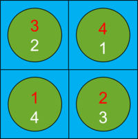
Sometimes the data accepted or provided by a solver may lie on a specific mesh type but follow an indexing that is different from this default. Consider the situation in the following figure:
The red numbers indicate the default indexing in this 2x2x1 regular Cartesian mesh. If our coupled solver would have the inverse indexing shown in white, we would have to account for that fact in the data transfer. The idea in the Cerberus coupling is to allow the coupled solvers to send and receive data in their preferred indexing, so that the coupled solvers do not have to rearrange data when sending or receiving it. This is achieved by the option to provide an indexing array as a part of a field template.
The indexing array, which needs to be sent if the indexing flag in the sent field template is set to 1 is simply an array of integers with the length of the array corresponding to the number of cells in the mesh and the contents of the array describing which solver index (white) corresponds to which global index (red). The first value of the array indicates the solver index corresponding to global index 1 and so on.
The indexing array for our 2x2 example above would thus be
4 3 2 1
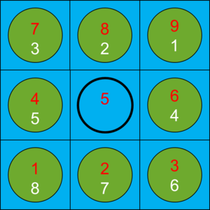
The indexing array can also account for the fact that the coupled solver will not accept or provide data for specific cell index/indices. If the coupled solver would only provide data for fuel rods and the geometry for the simulation would be as follows:
In this case the coupled solver does not consider the global cell 5 to be a part of its solution domain and thus will not provide or accept field data for that cell. Global cell 5 can be left un-indexed by setting the value 0 for it in the indexing array, which would now be
8 7 6 5 0 4 3 2 1
In such cases where some mesh cells are not indexed, the number of values for the field transferred between Cerberus and the solver will be reduced. In this case only 8 values would be transferred in the giveFieldData and takeFieldData calls.
Extending the previous example from 3x3x1 to 3x3x2 the indexing array might be
8 7 6 5 0 4 3 2 1 16 15 14 13 0 12 11 10 9
assuming that the indexing of the coupled solver on the upper axial layer is similar to that in the lower axial layer shown in the previous figure.
