Difference between revisions of "SMR startup simulation (outdated)"
(→Global variables during reactor startup) |
(→Global variables during reactor startup) |
||
| Line 1,438: | Line 1,438: | ||
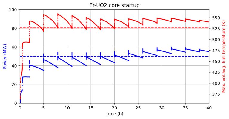
[[File:FuelT_40.png|frameless|x400px|Evolution of reactor power and maximum nodal fuel temperature during first 40 hours of reactor startup.]] | [[File:FuelT_40.png|frameless|x400px|Evolution of reactor power and maximum nodal fuel temperature during first 40 hours of reactor startup.]] | ||
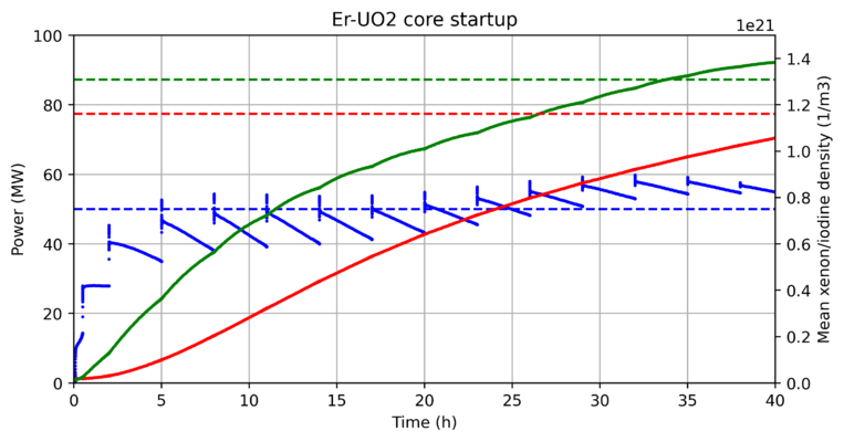
| − | The quick increase in reactor power after control rod movement is followed by a slow decrease in the reactor power (and maximum fuel temperature). This decrease is due to the increase in the xenon 135 concentrations, which take a long time to converge to equilibrium concentrations: | + | The quick increase in reactor power after control rod movement is followed by a slow decrease in the reactor power (and maximum fuel temperature). This decrease is due to the increase in the xenon 135 concentrations, which take a long time to converge to equilibrium concentrations (green color for I-135 and red for Xe-135): |
[[File:Poison_40.png|frameless|x400px|Evolution of reactor power and Xe-135 & I-135 nuclide densities during first 40 hours of reactor startup.]] | [[File:Poison_40.png|frameless|x400px|Evolution of reactor power and Xe-135 & I-135 nuclide densities during first 40 hours of reactor startup.]] | ||
| + | |||
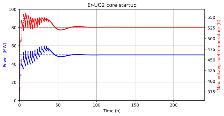
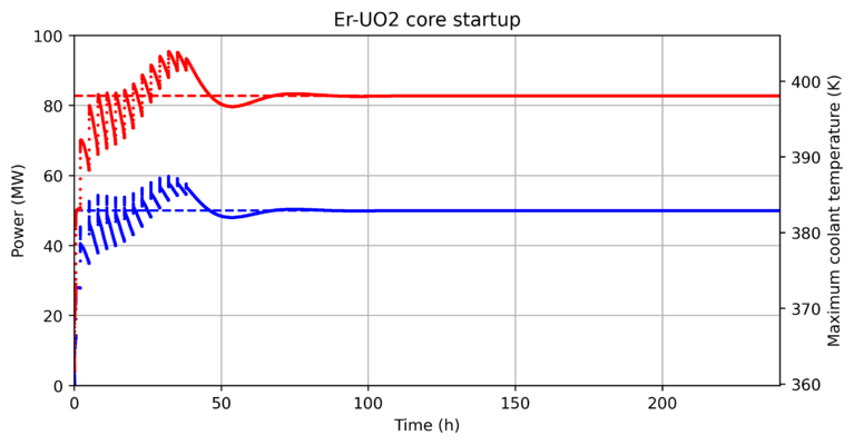
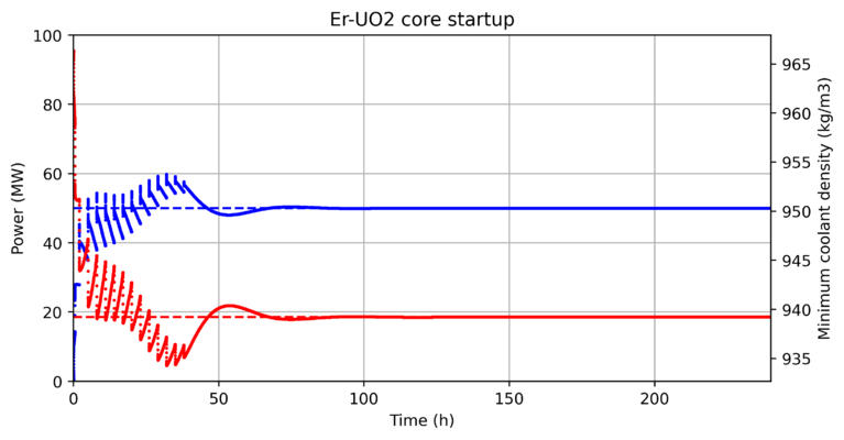
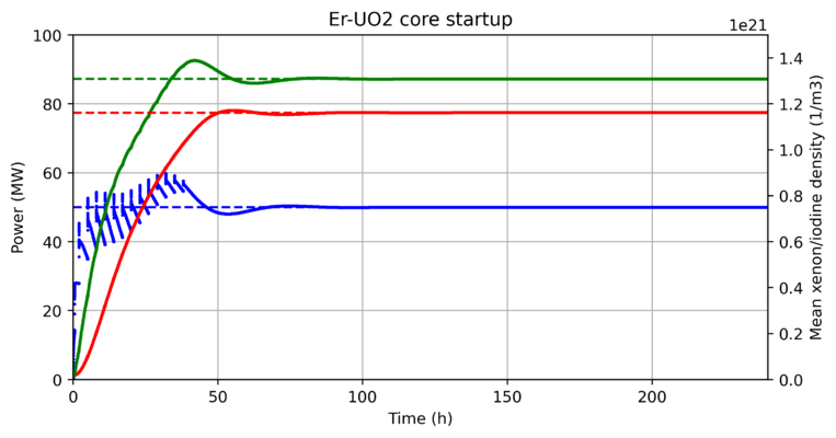
| + | The global variables do eventually converge to the steady state stationary values after some xenon oscillations: | ||
| + | |||
| + | [[File:FuelT_240.png|frameless|x400px|Evolution of reactor power and maximum nodal fuel temperature during the 240 hours of reactor startup.]] | ||
| + | [[File:CoolT_240.png|frameless|x400px|Evolution of reactor power and maximum nodal coolant temperature during the 240 hours of reactor startup.]] | ||
| + | [[File:CoolD_240.png|frameless|x400px|Evolution of reactor power and minimum nodal coolant density during the 240 hours of reactor startup.]] | ||
| + | [[File:Poison_240.png|frameless|x400px|Evolution of reactor power and Xe-135 & I-135 nuclide densities during the 240 hours of reactor startup.]] | ||
Revision as of 09:48, 9 September 2021
Contents
Overview
In order to test and demonstrate the time dependent calculation capabilities of the Kraken framework in a reasonably realistic context, a time dependent simulation was conducted of the initial rise to power of a small modular reactor (SMR) core. The simulation used the Ants nodal neutronics code to resolve the evolution of neutronics and the xenon fission poison chain in the system and the SUBCHANFLOW thermal hydraulics code to solve the coolant flow and heat transfer in fuel rods.
All of the input files are included as one archive here: File:SMR startup.tgz
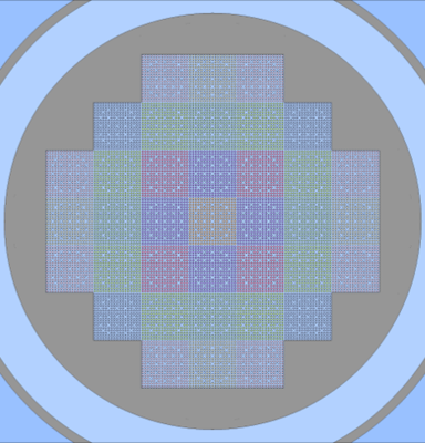
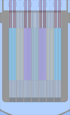
The modelled SMR is the same 37 assembly Er-UO2 fuelled core that has been previously used for the demonstration of the depletion capabilities of Kraken:
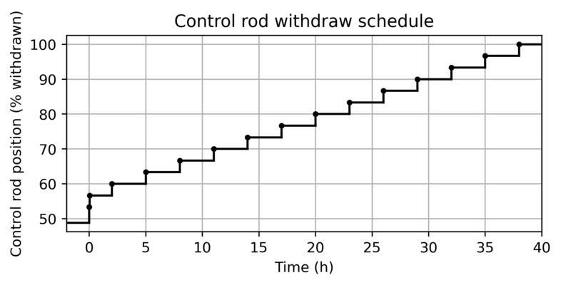
The transient starts from critical hot zero power (HZP) conditions (actually from 1 % power level) with all control rod banks at approximately 50 % insertion. The boron concentration in the coolant corresponds to the critical boron at all rods out (ARO) hot full power (HFP) conditions. The control rods are withdrawn from the core in a stepwise manner over 38 hours to allow for the accumulation of xenon in the core:
To reformulate the simulation setup:
- Evaluate (in a time-independent simulation) critical boron at hot full power all rods out conditions with convergence in
- Neutronics
- Thermal hydraulics
- Fuel temperature
- Xenon
- Using that critical boron, evaluate (in a time-independent simulation) critical control rod position at 1 % power level with convergence in
- Neutronics
- Thermal hydraulics
- Fuel temperature
- Xenon
- Save initial conditions from the 1 % power level time-independent calculation.
- Start a time dependent simulation from 1 % power level and slowly withdraw the control rods fully from the core.
If the time-independent and time-dependent calculation methodologies produce equivalent steady state solutions and have been correctly implemented, the simulation should (in the end) end up in the same state as the time-independent HFP ARO calculation.
Evaluating HFP ARO critical boron
The first part of the simulation is only needed here in order to obtain a more realistic and reasonable end state for the transient simulation by finding a realistic boron concentration for the coolant. The simulation is set up as a normal coupled steady state simulation between Ants and SUBCHANFLOW with Ants using its equilibrium xenon calculation mode and iterating the coolant boron concentration to reach a critical system. The system power is set to 50 MW, which corresponds to the nominal full power in the Er-UO2 core.
The Cerberus input used for the calculation is included below and is a rather simple coupled calculation input. It may be interesting to note that since Ants is developed in the Kraken context, many of the basic input data can be sent to Ants via Cerberus (control rod positions, system power, xenon calculation mode, iteration mode etc.). The same Ants input is actually used for all of the simulations here with the relevant parts of the Ants model being modified via Cerberus instead of in the Ants input file. Conversely, as SUBCHANFLOW is developed by KIT and the Kraken-coupling is achieved via a VTT written SUBCHANFLOW wrapper the amount of possible input data accessible via Cerberus is more limited and the steady state simulations use a (very slightly) different input file for SUBCHANFLOW than the transient simulation.
input.py: Cerberus input for HPF ARO boron iteration
from os import environ
from pathlib import Path

import numpy as np

import cerberus as cb
from cerberus.solvers import CodeInput
from cerberus.solvers import Solver
from cerberus.interpolation import Interpolator
from numpy.core.fromnumeric import size

# Verbosity for terminal output of Cerberus

cb.LOG.set_verbosity(1)

# Create and start solvers

solver_defs = [["SCF", environ["SCFWRAP_EXE_PATH"], [], ["../Inputs/scf/input_steady.txt"]],
               ["ANTS", environ["ANTS_EXE_PATH"], ["--cerberus","--port"], ["../Inputs/Ants.inp"]]]

solvers = {}

port_number = 2211

for name, solver_path, params, inputs in solver_defs:

    # Create input

    solver_input = CodeInput(name, inputs)

    # Create solver

    solver = Solver(name, solver_path, params)
    solver.input = solver_input
    solver.initialize(port_number)

    # Add to solver dict

    solvers[name] = solver

    port_number += 1

# Alias variables for solvers

scf = solvers["SCF"]
ants = solvers["ANTS"]

# Get SCF fields needed for coupled calculation

scf_cool_temperature = scf.get_transferrable("scf_of_cool_temperature_chan")
scf_cool_density = scf.get_transferrable("scf_of_cool_density_chan")
scf_fuel_temperature = scf.get_transferrable("scf_of_fuel_temperature_vol_ave")
scf_power = scf.get_transferrable("scf_if_fuel_power")

# Get Ants fields needed for coupled calculation

ants_cool_temperature = ants.get_transferrable("Ants_if_coolant_temperature")
ants_cool_density = ants.get_transferrable("Ants_if_coolant_density")
ants_fuel_temperature = ants.get_transferrable("Ants_if_fuel_temperature")
ants_power = ants.get_transferrable("Ants_of_supernode_power")
ants_boron = ants.get_transferrable("Ants_ov_boron")

# Create interpolators that handle data transfer between SCF and Ants

interp_ct = Interpolator.from_file(scf_cool_temperature,
                                   ants_cool_temperature,
                                   "../Inputs/scf_to_ants.txt")
interp_cd = Interpolator.from_file(scf_cool_density,
                                   ants_cool_density,
                                   "../Inputs/scf_to_ants.txt")
interp_ft = Interpolator.from_file(scf_fuel_temperature,
                                   ants_fuel_temperature,
                                   "../Inputs/scf_to_ants.txt")
interp_p = Interpolator.from_file(ants_power,
                                  scf_power,
                                  "../Inputs/ants_to_scf.txt")

################################################################################

# Setup some options for the Ants model

# 100 % power level (50 MW)

tra = ants.get_transferrable("Ants_iv_total_power")
tra.value_vec[0] = 50e6
tra.communicate()

# Equilibrium xenon (0 = zero, 1 = fixed, 2 = equilibrium, 3 = dynamic, 4 = depletion)

tra = ants.get_transferrable("Ants_iv_xenon_state")
tra.value_vec[0] = 2
tra.communicate()

# Control variable (iterate keff (1) or boron (2)?), here boron

tra = ants.get_transferrable("Ants_iv_control_variable")
tra.value_vec[0] = 2
tra.communicate()

# Initial value for keff

tra = ants.get_transferrable("Ants_iv_keff")
tra.value_vec[0] = 1.0
tra.communicate()

# Initial value for boron (ppm)

tra = ants.get_transferrable("Ants_iv_boron")
tra.value_vec[0] = 200.0
tra.communicate()

# Control rod position

height = 200.0

names = ["Ants_iv_cr_bank_height_CR2.1",
         "Ants_iv_cr_bank_height_CR2.2",
         "Ants_iv_cr_bank_height_CR2.3",
         "Ants_iv_cr_bank_height_CR2.4",
         "Ants_iv_cr_bank_height_CR4.1",
         "Ants_iv_cr_bank_height_CR4.2",
         "Ants_iv_cr_bank_height_CR4.3",
         "Ants_iv_cr_bank_height_CR4.4",
         "Ants_iv_cr_bank_height_CR6.1",
         "Ants_iv_cr_bank_height_CR6.2",
         "Ants_iv_cr_bank_height_CR6.3",
         "Ants_iv_cr_bank_height_CR6.4",
         "Ants_iv_cr_bank_height_CR6.5",
         "Ants_iv_cr_bank_height_CR6.6",
         "Ants_iv_cr_bank_height_CR6.7",
         "Ants_iv_cr_bank_height_CR6.8"]

for name in names:
    tra = ants.get_transferrable(name)
    tra.value_vec[0] = height
    tra.communicate()

################################################################################

# Initialize SCF power field (50 MW divided uniformly over SCF cells)

scf_power.value_vec = 50e6/scf_power.n_values*np.ones(scf_power.n_values)

################################################################################
################################################################################

# --- Coupled solution

max_iter = 50
for i in range(max_iter):
    # --- TH solution and communication

    scf_power.communicate()
    scf_power.write_simple(suffix_in=f"{i+1}")

    scf.solve()

    scf_cool_density.communicate()
    scf_cool_temperature.communicate()
    scf_fuel_temperature.communicate()

    # --- Transfers from SCF to Ants fields

    interp_ct.interpolate()
    interp_cd.interpolate()
    interp_ft.interpolate()

    # --- Neutronics solution and communication

    ants_cool_density.communicate()
    ants_cool_temperature.communicate()
    ants_fuel_temperature.communicate()

    ants.solve()

    ants_power.communicate()
    ants_boron.communicate()

    # --- Transfers from Ants to SCF

    interp_p.interpolate()

    print(f"Finished iteration {i+1}, boron is {ants_boron.value_vec[0]}")

# Choose field/value names to save
# (save HFP steady state fields so that we can compare our transient final state
#  to them)

to_save = ["Ants_ov_keff", "Ants_ov_boron",
           "Ants_if_fuel_temperature", "Ants_if_coolant_temperature",
           "Ants_if_coolant_density", "Ants_of_power",
           "Ants_of_number_density_xe135",
           "Ants_of_number_density_i135"]

# Output path. Create folder if necessary

output_path = Path(f"./output")
output_path.mkdir(exist_ok=True)
for name in to_save:
    tra = ants.get_transferrable(name)
    tra.communicate()
    tra.write_simple(suffix_in="final", folder_path=output_path)
As we can see from the Cerberus output, the coupled boron iteration convergences in a fast an orderly manner:
Part of Cerberus output for HPF ARO boron iteration
[...]
Finished iteration 1, boron is 228.22516244204832
Finished iteration 2, boron is 230.30442058650905
Finished iteration 3, boron is 183.3051192619623
Finished iteration 4, boron is 164.65050546552237
Finished iteration 5, boron is 157.30379476200793
Finished iteration 6, boron is 154.4821237790289
Finished iteration 7, boron is 153.3938241369474
Finished iteration 8, boron is 152.97112777867784
Finished iteration 9, boron is 152.8055417631124
Finished iteration 10, boron is 152.74065234503502
Finished iteration 11, boron is 152.7152600677249
Finished iteration 12, boron is 152.70531858398897
Finished iteration 13, boron is 152.70142257951275
Finished iteration 14, boron is 152.69989492716115
Finished iteration 15, boron is 152.69929592230528
Finished iteration 16, boron is 152.69906109692272
Finished iteration 17, boron is 152.698969052524
Finished iteration 18, boron is 152.69893297541552
Finished iteration 19, boron is 152.6989188350122
Finished iteration 20, boron is 152.69891329275947
Finished iteration 21, boron is 152.6989111207322
Finished iteration 22, boron is 152.69891026952354
Finished iteration 23, boron is 152.69890993601513
Finished iteration 24, boron is 152.698909805322
Finished iteration 25, boron is 152.6989097541711
Finished iteration 26, boron is 152.69890973416008
Finished iteration 27, boron is 152.69890972649966
Finished iteration 28, boron is 152.6989097235083
Finished iteration 29, boron is 152.69890972243354
Finished iteration 30, boron is 152.6989097220775
Finished iteration 31, boron is 152.69890972200204
Finished iteration 32, boron is 152.69890972199858
Finished iteration 33, boron is 152.6989097220187
Finished iteration 34, boron is 152.69890972213608
Finished iteration 35, boron is 152.69890972224186
Finished iteration 36, boron is 152.69890972236064
Finished iteration 37, boron is 152.69890972247714
Finished iteration 38, boron is 152.69890972253432
Finished iteration 39, boron is 152.69890972256997
Finished iteration 40, boron is 152.69890972269314
Finished iteration 41, boron is 152.6989097228652
Finished iteration 42, boron is 152.6989097229433
Finished iteration 43, boron is 152.69890972308616
Finished iteration 44, boron is 152.6989097232077
Finished iteration 45, boron is 152.69890972335665
Finished iteration 46, boron is 152.6989097234828
Finished iteration 47, boron is 152.69890972353284
Finished iteration 48, boron is 152.6989097236028
Finished iteration 49, boron is 152.69890972373645
Finished iteration 50, boron is 152.69890972385272
The critical boron for hot full power conditions is thus 152.69890972385272 ppm, which we can use as the coolant boron concentration for the second and third parts of the demonstration.
At the end of the iteration, Cerberus saves the fields corresponding to the converged HFP solution. These fields can be used as a reference solution for future comparisons.
We can also run a small script that extracts some relevant global data from the HFP fields, e.g. maximum temperatures and minimum densities:
get_HFP_values.py: Script for extracting global data from the output of the initial simulation
import numpy as np

data = np.loadtxt("./output/Ants_of_power.field_data_global.final", skiprows=1)
tot_power = np.nansum(data)

data = np.loadtxt("./output/Ants_if_coolant_temperature.field_data_global.final", skiprows=1)
max_coolT = np.nanmax(data)

data = np.loadtxt("./output/Ants_if_coolant_density.field_data_global.final", skiprows=1)
min_coolD = np.nanmin(data)

data = np.loadtxt("./output/Ants_of_number_density_xe135.field_data_global.final", skiprows=1)
mean_xenon = np.nanmean(data[np.where(data > 0)])

data = np.loadtxt("./output/Ants_of_number_density_i135.field_data_global.final", skiprows=1)
mean_iodine = np.nanmean(data[np.where(data > 0)])

data = np.loadtxt("./output/Ants_if_fuel_temperature.field_data_global.final", skiprows=1)
max_fuelT = np.nanmax(data)

fout = open("HFP_state.txt", "w")
fout.write("{:.4E} ".format(tot_power))
fout.write("{:.2f} ".format(max_coolT))
fout.write("{:.2f} ".format(min_coolD))
fout.write("{:.4E} ".format(mean_xenon))
fout.write("{:.4E} ".format(mean_iodine))
fout.write("{:.3f}\n".format(max_fuelT))
fout.close()
Evaluating critical control rod position at HZP fixed boron conditions
The next phase in the demonstration involves finding the critical control rod position for the HZP (1 % power) reactor using the coolant boron concentration obtained in the previous part.
The Cerberus input for the coupled critical control rod iteration is in many ways similar to the one we used for coupled critical boron iteration. However, whereas Ants can handle the iteration of the boron concentration internally, we need to write the control rod iteration to the Cerberus side.
The control rod iteration implemented here is very simple and straightforward. The process starts from a known supercritical control rod position (150 cm) and inserts the control rod with steps of 10 cm. When the reactor goes subcritical, the movement direction of the control rods is reversed and the control rod movement step is reduced to 10 % of the previous one. This process is repeated with direction changes and decreasing control rod movement step size until the reactor is critical within the specified threshold (0.01 pcm).
More intelligent and faster converging algorithms for critical control rod position could be used instead (as is done in the Kraken based reactor simulator), but this one was chosen here due to it being both simple to understand and implement.
At the end of the iteration, the initial conditions for the transient simulation are saved by Cerberus.
Cerberus input for HZP control rod iteration
from os import environ
from pathlib import Path

import numpy as np

import cerberus as cb
from cerberus.solvers import CodeInput
from cerberus.solvers import Solver
from cerberus.interpolation import Interpolator
from numpy.core.fromnumeric import size

# Verbosity for terminal output of Cerberus

cb.LOG.set_verbosity(1)

# Create and start solvers

solver_defs = [["SCF", environ["SCFWRAP_EXE_PATH"], [], ["../Inputs/scf/input_steady.txt"]],
               ["ANTS", environ["ANTS_EXE_PATH"], ["--cerberus","--port"], ["../Inputs/Ants.inp"]]]

solvers = {}

port_number = 2211

for name, solver_path, params, inputs in solver_defs:

    # Create input

    solver_input = CodeInput(name, inputs)

    # Create solver

    solver = Solver(name, solver_path, params)
    solver.input = solver_input
    solver.initialize(port_number)

    # Add to solver dict

    solvers[name] = solver

    port_number += 1

# Alias variables for solvers

scf = solvers["SCF"]
ants = solvers["ANTS"]

# Get SCF fields needed for coupled calculation

scf_cool_temperature = scf.get_transferrable("scf_of_cool_temperature_chan")
scf_cool_density = scf.get_transferrable("scf_of_cool_density_chan")
scf_fuel_temperature = scf.get_transferrable("scf_of_fuel_temperature_vol_ave")
scf_power = scf.get_transferrable("scf_if_fuel_power")

# Get Ants fields needed for coupled calculation

ants_cool_temperature = ants.get_transferrable("Ants_if_coolant_temperature")
ants_cool_density = ants.get_transferrable("Ants_if_coolant_density")
ants_fuel_temperature = ants.get_transferrable("Ants_if_fuel_temperature")
ants_power = ants.get_transferrable("Ants_of_supernode_power")
ants_boron = ants.get_transferrable("Ants_ov_boron")

# Create interpolators that handle data transfer between SCF and Ants

interp_ct = Interpolator.from_file(scf_cool_temperature,
                                   ants_cool_temperature,
                                   "../Inputs/scf_to_ants.txt")
interp_cd = Interpolator.from_file(scf_cool_density,
                                   ants_cool_density,
                                   "../Inputs/scf_to_ants.txt")
interp_ft = Interpolator.from_file(scf_fuel_temperature,
                                   ants_fuel_temperature,
                                   "../Inputs/scf_to_ants.txt")
interp_p = Interpolator.from_file(ants_power,
                                  scf_power,
                                  "../Inputs/ants_to_scf.txt")

################################################################################

# Setup some options for the Ants model

# 1 % power level (500 kW)

tra = ants.get_transferrable("Ants_iv_total_power")
tra.value_vec[0] = 500e3
tra.communicate()

# Equilibrium xenon (0 = zero, 1 = fixed, 2 = equilibrium, 3 = dynamic, 4 = depletion)

tra = ants.get_transferrable("Ants_iv_xenon_state")
tra.value_vec[0] = 2
tra.communicate()

# Control variable (iterate keff (1) or boron (2)?), here keff

tra = ants.get_transferrable("Ants_iv_control_variable")
tra.value_vec[0] = 1
tra.communicate()

# Initial value for keff

tra = ants.get_transferrable("Ants_iv_keff")
tra.value_vec[0] = 1.0
tra.communicate()

# Initial value for boron (ppm), from first part of the simulation

tra = ants.get_transferrable("Ants_iv_boron")
tra.value_vec[0] = 152.69890972385272
tra.communicate()

# Control rod position (initial guess)

cur_h = 150.0
delta_h = 10.0
prev_k = 1.1
direction = -1.0
num_iter = 3

cr_names = ["Ants_iv_cr_bank_height_CR2.1",
            "Ants_iv_cr_bank_height_CR2.2",
            "Ants_iv_cr_bank_height_CR2.3",
            "Ants_iv_cr_bank_height_CR2.4",
            "Ants_iv_cr_bank_height_CR4.1",
            "Ants_iv_cr_bank_height_CR4.2",
            "Ants_iv_cr_bank_height_CR4.3",
            "Ants_iv_cr_bank_height_CR4.4",
            "Ants_iv_cr_bank_height_CR6.1",
            "Ants_iv_cr_bank_height_CR6.2",
            "Ants_iv_cr_bank_height_CR6.3",
            "Ants_iv_cr_bank_height_CR6.4",
            "Ants_iv_cr_bank_height_CR6.5",
            "Ants_iv_cr_bank_height_CR6.6",
            "Ants_iv_cr_bank_height_CR6.7",
            "Ants_iv_cr_bank_height_CR6.8"]

for name in cr_names:
    tra = ants.get_transferrable(name)
    tra.value_vec[0] = cur_h
    tra.communicate()

################################################################################

# Initialize SCF power field (50 MW divided uniformly over SCF cells)

scf_power.value_vec = 50e6/scf_power.n_values*np.ones(scf_power.n_values)

################################################################################
################################################################################

# Coupled solution

while True:
    for i in range(num_iter):
        # --- TH solution and communication

        scf_power.communicate()
        scf_power.write_simple(suffix_in=f"{i+1}")

        scf.solve()

        scf_cool_density.communicate()
        scf_cool_temperature.communicate()
        scf_fuel_temperature.communicate()

        # --- Transfers from SCF to Ants fields

        interp_ct.interpolate()
        interp_cd.interpolate()
        interp_ft.interpolate()

        # --- Neutronics solution and communication

        ants_cool_density.communicate()
        ants_cool_temperature.communicate()
        ants_fuel_temperature.communicate()

        ants.solve()

        ants_power.communicate()
        ants_boron.communicate()

        # --- Transfers from Ants to SCF

        interp_p.interpolate()

    tra = ants.get_transferrable("Ants_ov_keff")
    tra.communicate()
    cur_k = tra.value_vec[0]

    print("Height is {}, keff is {} (based on {} coupled iterations)".format(cur_h, cur_k, num_iter))

    if (cur_k - 1)*(prev_k - 1) < 0:
        # --- Direction changes
        delta_h = delta_h/10.0
        direction *= -1
        prev_k = cur_k
        num_iter += 3

    if np.abs(cur_k - 1) < 1e-7:
        break

    cur_h += delta_h*direction

    # Move control rods to new position

    for name in cr_names:
        tra = ants.get_transferrable(name)
        tra.value_vec[0] = cur_h
        tra.communicate()

# Store final power field

scf_power.write_simple(suffix_in="final")

################################################################################
# Get dimensions from Ants

tra = ants.get_transferrable("Ants_ov_num_polynomial")
tra.communicate() # Get values from Ants
n_poly = tra.value_vec[0] # Get first value

tra = ants.get_transferrable("Ants_ov_num_group")
tra.communicate() # Get values from Ants
n_group = tra.value_vec[0] # Get first value

tra = ants.get_transferrable("Ants_ov_num_precursor_group")
tra.communicate() # Get values from Ants
n_prec_group = tra.value_vec[0] # Get first value

tra = ants.get_transferrable("Ants_ov_num_moment")
tra.communicate() # Get values from Ants
n_mom = tra.value_vec[0] # Get first value

################################################################################
# Store field/value names to save

to_save = ["Ants_ov_keff", "Ants_ov_boron",
           "Ants_if_coolant_temperature",
           "Ants_if_coolant_density",
           "Ants_if_fuel_temperature",
           "Ants_of_power",
           "Ants_of_number_density_i135",
           "Ants_of_number_density_xe135",
           "Ants_of_supernode_power"]

for poly_idx in range(n_poly):
    for group_idx in range(n_group):
        to_save.append(f"Ants_of_flux_expansion_coeff_poly_{poly_idx+1}_group_{group_idx+1}")
        to_save.append(f"Ants_of_fission_source_expansion_coeff_poly_{poly_idx+1}_group_{group_idx+1}")
    for group_idx in range(n_prec_group):
        to_save.append(f"Ants_of_precursor_expansion_coeff_poly_{poly_idx+1}_precursor_group_{group_idx+1}")
for group_idx in range(n_group):
    for mom_idx in range(n_mom):
        to_save.append(f"Ants_of_outcurrent_group_{group_idx+1}_moment_{mom_idx+1}")

# Output path. Create folder if necessary

output_path = Path(f"./output")
output_path.mkdir(exist_ok=True)
for name in to_save:
    tra = ants.get_transferrable(name)
    tra.communicate()
    tra.write_simple(suffix_in="final", folder_path=output_path)
The control rod iteration proceeds as expected converging in a reasonable manner:
Part of Cerberus output for HZP control rod iteration
[...]
Height is 150.0, keff is 1.012390300822608 (based on 3 coupled iterations)
Height is 140.0, keff is 1.0082079958086647 (based on 3 coupled iterations)
Height is 130.0, keff is 1.0029496683534684 (based on 3 coupled iterations)
Height is 120.0, keff is 0.9961290237278243 (based on 3 coupled iterations)
Height is 121.0, keff is 0.9966896419057593 (based on 6 coupled iterations)
Height is 122.0, keff is 0.9973041201566205 (based on 6 coupled iterations)
Height is 123.0, keff is 0.9980093145034636 (based on 6 coupled iterations)
Height is 124.0, keff is 0.998827315314074 (based on 6 coupled iterations)
Height is 125.0, keff is 0.9997878532518494 (based on 6 coupled iterations)
Height is 126.0, keff is 1.000257768448164 (based on 6 coupled iterations)
Height is 125.9, keff is 1.000208038391215 (based on 9 coupled iterations)
Height is 125.80000000000001, keff is 1.000158956010893 (based on 9 coupled iterations)
Height is 125.70000000000002, keff is 1.0001104993729535 (based on 9 coupled iterations)
Height is 125.60000000000002, keff is 1.000062656289768 (based on 9 coupled iterations)
Height is 125.50000000000003, keff is 1.0000154148864386 (based on 9 coupled iterations)
Height is 125.40000000000003, keff is 0.9999687635909442 (based on 9 coupled iterations)
Height is 125.41000000000004, keff is 0.9999734024943298 (based on 12 coupled iterations)
Height is 125.42000000000004, keff is 0.9999780471913975 (based on 12 coupled iterations)
Height is 125.43000000000005, keff is 0.9999826976988474 (based on 12 coupled iterations)
Height is 125.44000000000005, keff is 0.9999873540278879 (based on 12 coupled iterations)
Height is 125.45000000000006, keff is 0.9999920161897489 (based on 12 coupled iterations)
Height is 125.46000000000006, keff is 0.9999966841956976 (based on 12 coupled iterations)
Height is 125.47000000000007, keff is 1.0000013580570244 (based on 12 coupled iterations)
Height is 125.46900000000007, keff is 1.0000008904063895 (based on 15 coupled iterations)
Height is 125.46800000000006, keff is 1.0000004228144141 (based on 15 coupled iterations)
Height is 125.46700000000006, keff is 0.9999999552810814 (based on 15 coupled iterations)
Now we know that the reactor should be (very close to) critical at 1 % power level using critical boron concentration of 152.69890972385272 ppm and setting all control rods to the height of 125.467 cm.
Furthermore, we know that pulling all control rods out of the core should (eventually) lead the core to be critical at the HFP state (50 MW). We can test this in practice with a transient simulation starting from the HZP (1 % power) conditions where the control rods are slowly withdrawn from the core.
Transient simulation
The transient simulation itself is not a complex process, but consists of just a few different parts
- Initialization of solvers using fields saved from the HZP steady state solution.
- Time-integration loop over the whole simulation time.
- SUBCHANFLOW solution for thermal hydraulics
- Ants solution for neutronics
- Control rod movement at specific times
- Storing of relevant output data
- End of simulation
There are a couple of optional approaches taken here that make the input more complex:
- Adaptive timestepping to resolve both the fast power changes after control rod movement and the slow evolution of Iodine and Xenon over the 240 hours of simulation time.
- Acceleration of the fission poison solution in Ants to simulate long timesteps for poison evolution (up to several minutes) while only solving thermal hydraulics and neutronics with short timesteps (max 2.5 s) in order to keep the coupled solution stable.
- In-line evaluation of the 3D RMS differences between the time-dependent fields and the reference HZP and HFP steady state fields at each timestep. Storing all of the field data for each time step in order to do such comparisons in postprocessing would easily produce gigabytes of data.
input.py: Cerberus input for the transient simulation
from os import environ
from pathlib import Path
import time

import numpy as np

import cerberus as cb
from cerberus.solvers import CodeInput
from cerberus.solvers import Solver
from cerberus.interpolation import Interpolator

from krakentools.utils import seconds_to_timestring

# Verbosity for terminal output of Cerberus

cb.LOG.set_verbosity(1)

# Create and start solvers

solver_defs = [["SCF", environ["SCFWRAP_EXE_PATH"], [], ["../Inputs/scf/input_transient.txt"]],
               ["ANTS", environ["ANTS_EXE_PATH"], ["--cerberus","--port"], ["../Inputs/Ants.inp"]]]

solvers = {}

port_number = 2211

for name, solver_path, params, inputs in solver_defs:

    # Create input

    solver_input = CodeInput(name, inputs)

    # Create solver

    solver = Solver(name, solver_path, params)
    solver.input = solver_input
    solver.initialize(port_number)

    # Add to solver dict

    solvers[name] = solver

    port_number += 1

# Alias variables for solvers

scf = solvers["SCF"]
ants = solvers["ANTS"]

# Get SCF fields needed for coupled calculation

scf_cool_temperature = scf.get_transferrable("scf_of_cool_temperature_chan")
scf_cool_density = scf.get_transferrable("scf_of_cool_density_chan")
scf_fuel_temperature = scf.get_transferrable("scf_of_fuel_temperature_vol_ave")
scf_power = scf.get_transferrable("scf_if_fuel_power")

# Get Ants fields needed for coupled calculation

ants_cool_temperature = ants.get_transferrable("Ants_if_coolant_temperature")
ants_cool_density = ants.get_transferrable("Ants_if_coolant_density")
ants_fuel_temperature = ants.get_transferrable("Ants_if_fuel_temperature")
ants_power = ants.get_transferrable("Ants_of_supernode_power")
ants_2x2x2_power = ants.get_transferrable("Ants_of_power")
ants_boron = ants.get_transferrable("Ants_ov_boron")

ants_ff = ants.get_transferrable("Ants_iv_poison_ff")

ants_xenon = ants.get_transferrable("Ants_of_number_density_xe135")
ants_iodine = ants.get_transferrable("Ants_of_number_density_i135")

hfp_cool_temperature  = np.loadtxt("../1_HFP_ARO_boron_search/output/Ants_if_coolant_temperature.field_data_global.final", skiprows=1)
hfp_cool_density = np.loadtxt("../1_HFP_ARO_boron_search/output/Ants_if_coolant_density.field_data_global.final", skiprows=1)
hfp_fuel_temperature  = np.loadtxt("../1_HFP_ARO_boron_search/output/Ants_if_fuel_temperature.field_data_global.final", skiprows=1)
hfp_2x2x2_power  = np.loadtxt("../1_HFP_ARO_boron_search/output/Ants_of_power.field_data_global.final", skiprows=1)
hfp_xenon  = np.loadtxt("../1_HFP_ARO_boron_search/output/Ants_of_number_density_xe135.field_data_global.final", skiprows=1)
hfp_iodine = np.loadtxt("../1_HFP_ARO_boron_search/output/Ants_of_number_density_i135.field_data_global.final", skiprows=1)

hzp_cool_temperature  = np.loadtxt("../2_HZP_control_rod_search/output/Ants_if_coolant_temperature.field_data_global.final", skiprows=1)
hzp_cool_density = np.loadtxt("../2_HZP_control_rod_search/output/Ants_if_coolant_density.field_data_global.final", skiprows=1)
hzp_fuel_temperature  = np.loadtxt("../2_HZP_control_rod_search/output/Ants_if_fuel_temperature.field_data_global.final", skiprows=1)
hzp_2x2x2_power  = np.loadtxt("../2_HZP_control_rod_search/output/Ants_of_power.field_data_global.final", skiprows=1)
hzp_xenon  = np.loadtxt("../2_HZP_control_rod_search/output/Ants_of_number_density_xe135.field_data_global.final", skiprows=1)
hzp_iodine = np.loadtxt("../2_HZP_control_rod_search/output/Ants_of_number_density_i135.field_data_global.final", skiprows=1)

# Create interpolators that handle data transfer between SCF and Ants

interp_ct = Interpolator.from_file(scf_cool_temperature,
                                   ants_cool_temperature,
                                   "../Inputs/scf_to_ants.txt")
interp_cd = Interpolator.from_file(scf_cool_density,
                                   ants_cool_density,
                                   "../Inputs/scf_to_ants.txt")
interp_ft = Interpolator.from_file(scf_fuel_temperature,
                                   ants_fuel_temperature,
                                   "../Inputs/scf_to_ants.txt")
interp_p = Interpolator.from_file(ants_power,
                                  scf_power,
                                  "../Inputs/ants_to_scf.txt")

################################################################################

# Setup some options for the Ants model

# Dynamic xenon (0 = zero, 1 = fixed, 2 = equilibrium, 3 = dynamic, 4 = depletion)

tra = ants.get_transferrable("Ants_iv_xenon_state")
tra.value_vec[0] = 3
tra.communicate()

# Initial value for keff (from initial conditions)

tra = ants.get_transferrable("Ants_iv_keff")
tra.value_vec[0] = 0.9999999552810815
tra.communicate()

# Initial value for boron (ppm), from first part of the simulation

tra = ants.get_transferrable("Ants_iv_boron")
tra.value_vec[0] = 152.69890972385272
tra.communicate()

# Initial control rod position

cur_h = 125.467

cr_names = ["Ants_iv_cr_bank_height_CR2.1",
            "Ants_iv_cr_bank_height_CR2.2",
            "Ants_iv_cr_bank_height_CR2.3",
            "Ants_iv_cr_bank_height_CR2.4",
            "Ants_iv_cr_bank_height_CR4.1",
            "Ants_iv_cr_bank_height_CR4.2",
            "Ants_iv_cr_bank_height_CR4.3",
            "Ants_iv_cr_bank_height_CR4.4",
            "Ants_iv_cr_bank_height_CR6.1",
            "Ants_iv_cr_bank_height_CR6.2",
            "Ants_iv_cr_bank_height_CR6.3",
            "Ants_iv_cr_bank_height_CR6.4",
            "Ants_iv_cr_bank_height_CR6.5",
            "Ants_iv_cr_bank_height_CR6.6",
            "Ants_iv_cr_bank_height_CR6.7",
            "Ants_iv_cr_bank_height_CR6.8"]

for name in cr_names:
    tra = ants.get_transferrable(name)
    tra.value_vec[0] = cur_h
    tra.communicate()

################################################################################
# --- Setup and initialize the required fields

to_initialize = [(scf, "scf_if_fuel_power"),
                 (ants, "Ants_if_coolant_temperature"),
                 (ants, "Ants_if_coolant_density"),
                 (ants, "Ants_if_fuel_temperature"),
                 (ants, "Ants_of_number_density_xe135"),
                 (ants, "Ants_of_number_density_i135"),]

################################################################################
# Get dimensions from Ants

tra = ants.get_transferrable("Ants_ov_num_polynomial")
tra.communicate() # Get values from Ants
n_poly = tra.value_vec[0] # Get first value

tra = ants.get_transferrable("Ants_ov_num_group")
tra.communicate() # Get values from Ants
n_group = tra.value_vec[0] # Get first value

tra = ants.get_transferrable("Ants_ov_num_precursor_group")
tra.communicate() # Get values from Ants
n_prec_group = tra.value_vec[0] # Get first value

tra = ants.get_transferrable("Ants_ov_num_moment")
tra.communicate() # Get values from Ants
n_mom = tra.value_vec[0] # Get first value

################################################################################
# Store field/value names to save

to_save = ["Ants_ov_keff", "Ants_ov_boron",
           "Ants_if_coolant_temperature",
           "Ants_if_coolant_density",
           "Ants_if_fuel_temperature",
           "Ants_of_supernode_power",
           "Ants_of_power",
           "Ants_of_number_density_xe135",
           "Ants_of_number_density_i135"]

for poly_idx in range(n_poly):
    for group_idx in range(n_group):
        to_save.append(f"Ants_of_flux_expansion_coeff_poly_{poly_idx+1}_group_{group_idx+1}")
        to_save.append(f"Ants_of_fission_source_expansion_coeff_poly_{poly_idx+1}_group_{group_idx+1}")
        to_initialize.append((ants, f"Ants_of_flux_expansion_coeff_poly_{poly_idx+1}_group_{group_idx+1}"))
        to_initialize.append((ants, f"Ants_of_fission_source_expansion_coeff_poly_{poly_idx+1}_group_{group_idx+1}"))
    for group_idx in range(n_prec_group):
        to_save.append(f"Ants_of_precursor_expansion_coeff_poly_{poly_idx+1}_precursor_group_{group_idx+1}")
        to_initialize.append((ants, f"Ants_of_precursor_expansion_coeff_poly_{poly_idx+1}_precursor_group_{group_idx+1}"))

for group_idx in range(n_group):
    for mom_idx in range(n_mom):
        to_save.append(f"Ants_of_outcurrent_group_{group_idx+1}_moment_{mom_idx+1}")
        to_initialize.append((ants, f"Ants_of_outcurrent_group_{group_idx+1}_moment_{mom_idx+1}"))

# --- Initialize all fields that need to be initialized

for solver, tra_name in to_initialize:
    out_values = np.loadtxt(f"../2_HZP_control_rod_search/output/{tra_name}.field_data_global.final", skiprows=1)
    out_values[np.where(np.isnan(out_values))] = 0
    in_name = tra_name.replace("_of_", "_if_")
    tra = solver.get_transferrable(in_name)
    tra.value_vec = 1.0*out_values
    tra.communicate()

################################################################################
################################################################################

# Calculate initial steady state solution for SUBCHANFLOW based on HZP power field

scf.read_restart()


# Setup schedule for control rod movements

times_and_heights = [(5*60, 130), # First movement at five minutes
                     (30*60, 135), # Then at half an hour
                     (2*60*60, 140),
                     (5*60*60, 145),
                     (8*60*60, 150),
                     (11*60*60, 155),
                     (14*60*60, 160),
                     (17*60*60, 165),
                     (20*60*60, 170),
                     (23*60*60, 175),
                     (26*60*60, 180),
                     (29*60*60, 185),
                     (32*60*60, 190),
                     (35*60*60, 195),
                     (38*60*60, 200),
                     (1000*60*60, 200)]

# Time loop (fission poisons get accelerated so they have their own time)

solver_dt = 0.1
poison_dt = 0.1
end_time = 240*60*60.0

soon = False

poison_t = 0

beginning = time.time()

fout     = open("resu.txt", "w")
hzp_diff = open("Dhzp.txt", "w")
hfp_diff = open("Dhfp.txt", "w")

while(poison_t < end_time):
    t0, t1 = scf.return_current_time_interval()
    #print(f"Current t0 = {t0} t1 = {t1}")

    t0, t1_scf = scf.suggest_next_time_interval()
    #print(f"Suggested t0 = {t0} t1 = {t1_scf} ({solver_dt}/{poison_dt})")

    if t1_scf > t0 + poison_dt:
        t1_scf = t0 + poison_dt
    t1 = t0 + solver_dt

    if t0 == 0:
        scf.set_current_time_interval(t0, t1)
        ants.set_current_time_interval(t0, t1)
    else:
        scf.advance_to_time_interval(t0, t1)
        ants.advance_to_time_interval(t0, t1)

    t0, t1 = scf.return_current_time_interval()

    print(f"\nTime step from {poison_t:.3f} s with a length of {poison_dt:.3f} s")
    print(f"Xenon acceleration factor is {poison_dt/solver_dt:.2f}")

    poison_t += poison_dt


    # --- TH solution and communication

    scf_power.communicate()

    scf.solve()

    scf_cool_density.communicate()
    scf_cool_temperature.communicate()
    scf_fuel_temperature.communicate()

    # --- Transfers from SCF to Ants fields

    interp_ct.interpolate()
    interp_cd.interpolate()
    interp_ft.interpolate()

    # --- Neutronics solution and communication

    ants_cool_density.communicate()
    ants_cool_temperature.communicate()
    ants_fuel_temperature.communicate()


    ants.solve()
    num_iter = 1
    while ants.solve_return != 2:
        ants.solve()
        num_iter += 1
        if num_iter == 15:
           break

    ants_power.communicate()
    ants_2x2x2_power.communicate()
    ants_xenon.communicate()
    ants_iodine.communicate()

    # --- Transfers from Ants to SCF

    interp_p.interpolate()

    # --- Output from end of timestep

    tot_power = np.nansum(ants_power.value_vec)
    max_coolT = np.nanmax(ants_cool_temperature.value_vec)
    min_coolD = np.nanmin(ants_cool_density.value_vec)
    mean_xenon = np.nanmean(ants_xenon.value_vec[np.where(ants_xenon.value_vec > 0)])
    mean_iodine = np.nanmean(ants_iodine.value_vec[np.where(ants_iodine.value_vec > 0)])
    max_fuelT = np.nanmax(ants_fuel_temperature.value_vec)

    print("Current reactor power is {:.2E} W".format(tot_power))
    print("Took {} outer iterations for Ants".format(num_iter))

    fout.write("{:.4f} ".format(poison_t))
    fout.write("{:.4f} ".format(t1))
    fout.write("{:.2f} ".format(cur_h))
    fout.write("{:.4E} ".format(tot_power))
    fout.write("{:.2f} ".format(max_coolT))
    fout.write("{:.2f} ".format(min_coolD))
    fout.write("{:.3f} ".format(max_fuelT))
    fout.write("{:.4E} ".format(mean_xenon))
    fout.write("{:.4E}\n".format(mean_iodine))

    fout.flush()

    # --- RMS differences in fields compared to HZP steady state solution

    to_compare = ((hzp_2x2x2_power, ants_2x2x2_power),
                  (hzp_cool_temperature, ants_cool_temperature),
                  (hzp_cool_density, ants_cool_density),
                  (hzp_fuel_temperature, ants_fuel_temperature),
                  (hzp_xenon, ants_xenon),
                  (hzp_iodine, ants_iodine))

    hzp_diff.write("{:.4f} ".format(poison_t))
    for ref, cur in to_compare:
        cur = cur.value_vec
        delta =  (cur - ref)
        rdelta = delta[np.where(ref > 0)]/ref[np.where(ref > 0)]
        rms_diff = np.sqrt(np.mean(rdelta**2))

        hzp_diff.write("{:.4E} ".format(rms_diff))

    hzp_diff.write("\n")
    hzp_diff.flush()

    # --- RMS differences in fields compared to HFP steady state solution

    to_compare = ((hfp_2x2x2_power, ants_2x2x2_power),
                  (hfp_cool_temperature, ants_cool_temperature),
                  (hfp_cool_density, ants_cool_density),
                  (hfp_fuel_temperature, ants_fuel_temperature),
                  (hfp_xenon, ants_xenon),
                  (hfp_iodine, ants_iodine))

    hfp_diff.write("{:.4f} ".format(poison_t))
    for ref, cur in to_compare:
        cur = cur.value_vec
        delta =  (cur - ref)
        rdelta = delta[np.where(ref > 0)]/ref[np.where(ref > 0)]
        rms_diff = np.sqrt(np.mean(rdelta**2))

        hfp_diff.write("{:.4E} ".format(rms_diff))

    hfp_diff.write("\n")
    hfp_diff.flush()

    # --- Move control rod if needed

    next_t = times_and_heights[0][0]
    if poison_t > next_t:
        soon = False
        next_t, next_h = times_and_heights.pop(0)

        cur_h = next_h
        output_path = Path(f"./{cur_h}")
        output_path.mkdir(exist_ok=True)
        for name in to_save:
            tra = ants.get_transferrable(name)
            tra.communicate()
            tra.write_simple(suffix_in="final", folder_path=output_path)

        poison_dt = 5e-3

        names = ["Ants_iv_cr_bank_height_CR2.1",
                 "Ants_iv_cr_bank_height_CR2.2",
                 "Ants_iv_cr_bank_height_CR2.3",
                 "Ants_iv_cr_bank_height_CR2.4",
                 "Ants_iv_cr_bank_height_CR4.1",
                 "Ants_iv_cr_bank_height_CR4.2",
                 "Ants_iv_cr_bank_height_CR4.3",
                 "Ants_iv_cr_bank_height_CR4.4",
                 "Ants_iv_cr_bank_height_CR6.1",
                 "Ants_iv_cr_bank_height_CR6.2",
                 "Ants_iv_cr_bank_height_CR6.3",
                 "Ants_iv_cr_bank_height_CR6.4",
                 "Ants_iv_cr_bank_height_CR6.5",
                 "Ants_iv_cr_bank_height_CR6.6",
                 "Ants_iv_cr_bank_height_CR6.7",
                 "Ants_iv_cr_bank_height_CR6.8"]

        for name in names:
            tra = ants.get_transferrable(name)
            tra.value_vec[0] = cur_h
            tra.communicate()
    else:
        # --- Control rod was not moved, check if we need to move it soon
        #     and reduce timestep length

        if (next_t - poison_t)/poison_dt < 10:

            soon = True

            # --- Divide previous timestep length by 1.5

            poison_dt = poison_dt/1.50

            # --- Minimum timestep length before control rod movement is 1.0 s

            if poison_dt < 1.0:
                poison_dt = 1.0

        elif not soon:
            # --- If there is no control rod movement coming up, increase
            #     timestep length by 30 %

            poison_dt = 1.3*poison_dt

            # --- Maximum timestep to use for poison calculation

            if poison_dt > 3*60:
                poison_dt = 3*60

    # --- Explicit neutronics - TH coupling becomes unstable with timesteps
    #     longer than couple of seconds. Handle longer timesteps with xenon
    #     acceleration instead. Neutronics and TH should already be close to
    #     converged

    if poison_dt > 2.5:
        ants_ff.value_vec[0] = poison_dt/2.5
        solver_dt = 2.5
    else:
        ants_ff.value_vec[0] = 1.0
        solver_dt = poison_dt

    # --- Send xenon acceleration (fast forward) factor to Ants

    ants_ff.communicate()

fout.close()
hzp_diff.close()
hfp_diff.close()

# --- Print simulation time for solvers

print()
print(f"Ants took {seconds_to_timestring(ants.solution_timer._elapsed_time)}")
print(f"SCF took {seconds_to_timestring(scf.solution_timer._elapsed_time)}")
elapsed = time.time() - beginning
print(f"Total time was {seconds_to_timestring(elapsed)}")

# Output path. Create folder if necessary
output_path = Path(f"./output")
output_path.mkdir(exist_ok=True)
for name in to_save:
    tra = ants.get_transferrable(name)
    tra.communicate()
    tra.write_simple(suffix_in="final", folder_path=output_path)
Running the input solves the time-dependent evolution of the reactor over 240 hours. Control rod movements are finished after 38 hours.
Part of Cerberus output for the transient simulation
[...]

Time step from 0.000 s with a length of 0.100 s
Xenon acceleration factor is 1.00
Current reactor power is 5.00E+05 W
Took 2 outer iterations for Ants

Time step from 0.100 s with a length of 0.130 s
Xenon acceleration factor is 1.00
Current reactor power is 5.00E+05 W
Took 1 outer iterations for Ants

[...]

Time step from 863882.617 s with a length of 180.000 s
Xenon acceleration factor is 72.00
Current reactor power is 5.00E+07 W
Took 1 outer iterations for Ants

Ants took 4 h 0 min
SCF took 7 min 21 s
Total time was 5 h 36 min
The 240 hours of reactor operation are simulated using a total of 6273 time steps. Most of the time (70 %) is taken by the Ants solution, although a significant amount of time (25 %) also goes to field transfers and data processing outside of the solve-commands given to the two solvers,
Postprocessing
Now, the remaining question is whether
- The time-dependent solution is stationary in the initial HZP (1 % power) reactor before the first control rod movement.
- The time-dependent solution ends up in the same HFP ARO state as the time-independent solution.
Stationary HZP reactor
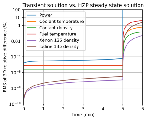
The RMS difference between the 3D fields from the time-independent HZP simulation and the time-dependent 3D fields from the transient simulation were evaluated and stored during the transient simulation. Now we only need to plot those RMS differences to see whether they stay small and close to constant during the initial part of the transient simulation.
HZP_diff.py: Plotting the difference between the time-independent HZP solution and the start of the time-dependent simulation
import matplotlib as mpl
import matplotlib.pyplot as plt

results = np.loadtxt("./Dhzp.txt")

t   = results[:,0]/60
dP  = results[:,1]*100
dTc = results[:,2]*100
dRc = results[:,3]*100
dTf = results[:,4]*100
dXe = results[:,5]*100
dI  = results[:,6]*100


fig, ax = plt.subplots()
fig.set_size_inches(5.0, 4.0)

ax.grid(True)

ax.plot(t, dP, label="Power")
ax.plot(t, dTc, label="Coolant temperature")
ax.plot(t, dRc, label="Coolant density")
ax.plot(t, dTf, label="Fuel temperature")
ax.plot(t, dXe, label="Xenon 135 density")
ax.plot(t, dI, label="Iodine 135 density")

ax.set_xlabel("Time (min)")
ax.set_yscale("log")
ax.set_ylim((1e-10, 100))
ax.set_xlim((0, 6))
ax.set_ylabel("RMS of 3D relative difference (%)")
ax.set_title("Transient solution vs. HZP steady state solution")

ax.set_yticks((1e-10, 1e-8, 1e-6, 1e-4, 1e-2, 1, 10, 100))
ax.set_yticklabels(("$10^{-10}$","$10^{-8}$","$10^{-6}$","$10^{-4}$","0.01","1", "10", "100"))

ax.legend(loc="upper left")
fig.savefig("./HZP_diff.png", bbox_inches="tight",dpi=400)

plt.close(fig)
The RMS relative differences between the 3D fields from steady state HZP reactor and the beginning of the transient simulation are plotted below:
As the simulation starts from the HZP fields the RMS relative differences are very small at the beginning of the simulation (around 1e-5 % i.e. 0.00001 %). The power is practically constant, although not exactly. This is most likely due to limited numerical precision in the initialization of the solution. Even then, the relative RMS difference in the 3D nodal power field is below 0.0001 % after 5 minutes of transient simulation.
After the first control rod withdrawal at 5 minutes the transient solution diverges from the HZP state as expected.
Global variables during reactor startup
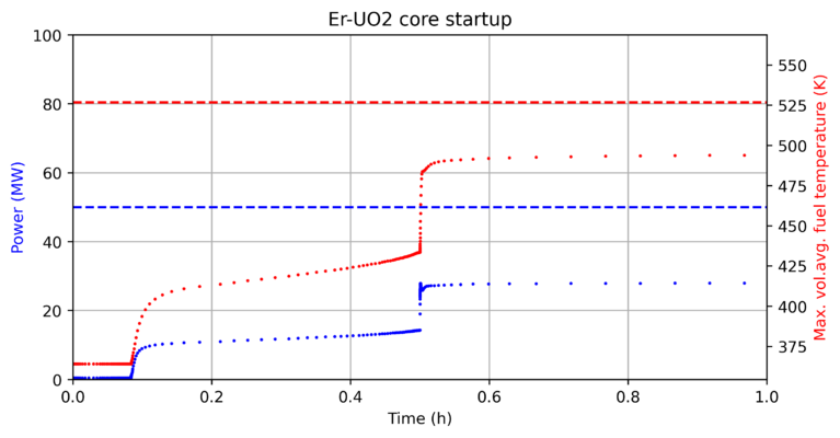
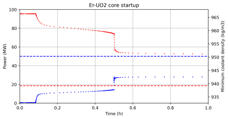
We can plot the global reactor power and some global variables of interest during the reactor startup to observe the phenomena occurring during reactor startup:
plot.py: Plotting the evolution of global variables during reactor startup
import matplotlib as mpl
import matplotlib.pyplot as plt

results = np.loadtxt("./resu.txt")

t = results[:,0]/60/60
P = results[:,3]/1e6
Tc = results[:,4]
Rc = results[:,5]
Tf = results[:,6]
Xe = results[:,7]
I  = results[:,8]

#
# Get reference data saved from HFP simulation
#

HFP_data = np.loadtxt("../1_HFP_ARO_boron_search/HFP_state.txt")

ref_P, ref_Tc, ref_Rc, ref_Xe, ref_I, ref_Tf = HFP_data

#
#
#

fig, ax = plt.subplots()
fig.set_size_inches(8.0, 4.0)
ax2 = ax.twinx()

ax.plot(t, P, "b.", markersize=2)
ax2.plot(t, Tf, "r.", markersize=2)
ax.plot((0, t[-1]), (ref_P/1e6, ref_P/1e6), "b--")
ax2.plot((0, t[-1]), (ref_Tf, ref_Tf), "r--")

ax.set_xlabel("Time (h)")
ax.set_ylim((0, 100))
ax.set_ylabel("Power (MW)", color="b")
ax2.set_ylabel("Max. vol.avg. fuel temperature (K)", color="r")
ax.set_title("Er-UO2 core startup")

ax.grid(True)
ax.set_xlim((0, 1))
fig.savefig("./FuelT_1.png", bbox_inches="tight",dpi=400)
ax.set_xlim((0, 40))
fig.savefig("./FuelT_40.png", bbox_inches="tight",dpi=400)
ax.set_xlim((0, 240))
fig.savefig("./FuelT_240.png", bbox_inches="tight",dpi=400)

plt.close(fig)

#
#
#

fig, ax = plt.subplots()
fig.set_size_inches(8.0, 4.0)

ax2 = ax.twinx()

ax.plot(t, P, "b.", markersize=2)
ax2.plot(t, Tc, "r.", markersize=2)
ax.plot((0, t[-1]), (ref_P/1e6, ref_P/1e6), "b--")
ax2.plot((0, t[-1]), (ref_Tc, ref_Tc), "r--")

ax.set_xlabel("Time (h)")
ax.set_ylim((0, 100))
ax.set_ylabel("Power (MW)")
ax2.set_ylabel("Maximum coolant temperature (K)")
ax.set_title("Er-UO2 core startup")

ax.grid(True)
ax.set_xlim((0, 1))
fig.savefig("./CoolT_1.png", bbox_inches="tight",dpi=400)
ax.set_xlim((0, 40))
fig.savefig("./CoolT_40.png", bbox_inches="tight",dpi=400)
ax.set_xlim((0, 240))
fig.savefig("./CoolT_240.png", bbox_inches="tight",dpi=400)

plt.close(fig)

#
#
#

fig, ax = plt.subplots()
fig.set_size_inches(8.0, 4.0)

ax2 = ax.twinx()

ax.plot(t, P, "b.", markersize=2)
ax2.plot(t, Rc, "r.", markersize=2)
ax.plot((0, t[-1]), (ref_P/1e6, ref_P/1e6), "b--")
ax2.plot((0, t[-1]), (ref_Rc, ref_Rc), "r--")

ax.set_xlabel("Time (h)")
ax.set_ylim((0, 100))
ax.set_ylabel("Power (MW)")
ax2.set_ylabel("Minimum coolant density (kg/m3)")
ax.set_title("Er-UO2 core startup")

ax.grid(True)
ax.set_xlim((0, 1))
fig.savefig("./CoolD_1.png", bbox_inches="tight",dpi=400)
ax.set_xlim((0, 40))
fig.savefig("./CoolD_40.png", bbox_inches="tight",dpi=400)
ax.set_xlim((0, 240))
fig.savefig("./CoolD_240.png", bbox_inches="tight",dpi=400)

plt.close(fig)

#
#
#

fig, ax = plt.subplots()
fig.set_size_inches(8.0, 4.0)

ax2 = ax.twinx()

ax.plot(t, P, "b.", markersize=2)
ax2.plot(t, Xe, "r.", markersize=2)
ax2.plot(t, I, "g.", markersize=2)

ax.plot((0, t[-1]), (ref_P/1e6, ref_P/1e6), "b--")
ax2.plot((0, t[-1]), (ref_Xe, ref_Xe), "r--")
ax2.plot((0, t[-1]), (ref_I, ref_I), "g--")

ax.set_xlabel("Time (h)")
ax.set_ylim((0, 100))
ax2.set_ylim((0, 1.5e21))
ax.set_ylabel("Power (MW)")
ax2.set_ylabel("Mean xenon/iodine density (1/m3)")
ax.set_title("Er-UO2 core startup")

ax.grid(True)
ax.set_xlim((0, 1))
fig.savefig("./Poison_1.png", bbox_inches="tight",dpi=400)
ax.set_xlim((0, 40))
fig.savefig("./Poison_40.png", bbox_inches="tight",dpi=400)
ax.set_xlim((0, 240))
fig.savefig("./Poison_240.png", bbox_inches="tight",dpi=400)
plt.close(fig)We plot the evolution of these global variables during 1, 40 and 240 hours. In addition to plotting the time-dependent values, dashed horizontal lines are plotted to include the values of these global variables in the time-independent HFP ARO simulation:
The control rod movements at 5 minutes and 30 minutes result in an increase in power and a quick increase in maximum fuel temperature. This is reflected in the minimum coolant density:
The control rod movements happen during the first 38 hours of the simulation:
The quick increase in reactor power after control rod movement is followed by a slow decrease in the reactor power (and maximum fuel temperature). This decrease is due to the increase in the xenon 135 concentrations, which take a long time to converge to equilibrium concentrations (green color for I-135 and red for Xe-135):
The global variables do eventually converge to the steady state stationary values after some xenon oscillations:
