Difference between revisions of "Kharon theory manual"
Ville Hovi (talk | contribs) (→References) |
Ville Hovi (talk | contribs) (→References) |
||
| Line 1,797: | Line 1,797: | ||
<ref name="Kunz1998"> Kunz, R. F., Siebert, B. W., Cope, W. K., Foster, N. F., Antal, S. P., Ettorre, S. M., A coupled phasic exchange algorithm for three–dimensional multi–field analysis of heated flows with mass transfer. Computers & Fluids 27 (7), pp. 741–768, 1998. </ref> | <ref name="Kunz1998"> Kunz, R. F., Siebert, B. W., Cope, W. K., Foster, N. F., Antal, S. P., Ettorre, S. M., A coupled phasic exchange algorithm for three–dimensional multi–field analysis of heated flows with mass transfer. Computers & Fluids 27 (7), pp. 741–768, 1998. </ref> | ||
<ref name="VasquezIvanov2000"> Vasquez, S. A., Ivanov, V. A., A phase coupled method for solving multiphase problems in unstructured meshes. In: Proceedings of ASME FEDSM’00: ASME 2000 fluids engineering division summer meeting, Boston. pp. 743-748, 2000. </ref> | <ref name="VasquezIvanov2000"> Vasquez, S. A., Ivanov, V. A., A phase coupled method for solving multiphase problems in unstructured meshes. In: Proceedings of ASME FEDSM’00: ASME 2000 fluids engineering division summer meeting, Boston. pp. 743-748, 2000. </ref> | ||
| − | <ref name=" | + | <ref name="Incropera2002a"> Incropera, F. P., DeWitt, D. P., Fundamentals of Heat and Mass Transfer, Chapter 8, p. 470, eq. 8.19. John Wiley & Sons, Inc. 2002. </ref> |
| − | <ref name=" | + | <ref name="Incropera2002b"> Incropera, F. P., DeWitt, D. P., Fundamentals of Heat and Mass Transfer, Chapter 8, p. 470, eq. 8.21. John Wiley & Sons, Inc. 2002. </ref> |
<ref name="KurulPodowski1991"> Kurul, N., Podowski, M. Z., On the Modeling of Multidimensional Effects in Boiling Channels. In: ANS Proceedings of 1991 National Heat Transfer Conference, Minneapolis, Minnesota, Vol. 5. pp. 30-40, 1991. ISBN: 0-89448-162-2 </ref> | <ref name="KurulPodowski1991"> Kurul, N., Podowski, M. Z., On the Modeling of Multidimensional Effects in Boiling Channels. In: ANS Proceedings of 1991 National Heat Transfer Conference, Minneapolis, Minnesota, Vol. 5. pp. 30-40, 1991. ISBN: 0-89448-162-2 </ref> | ||
<ref name="DelValleKenning1985"> Del Valle M., V. H., Kenning, D. B. R., Subcooled flow boiling at high heat flux. Int. J. Heat Mass Transfer, Vol. 28, No. 10, pp.1907-1920, 1985. </ref> | <ref name="DelValleKenning1985"> Del Valle M., V. H., Kenning, D. B. R., Subcooled flow boiling at high heat flux. Int. J. Heat Mass Transfer, Vol. 28, No. 10, pp.1907-1920, 1985. </ref> | ||
Revision as of 10:24, 1 April 2019
Contents
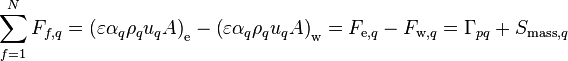
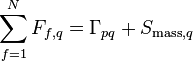
Conservation of Mass

Steady one-dimensional conservation of mass (of phase q) is given through the following relation
-

(1)
Equation 1 is discretized for an interior cell, shown in Figure 1, by volume integration over cell P.
-
![\Leftrightarrow \iiint\limits_V \left[\nabla\cdot\left(\varepsilon \alpha_q \rho_q u_q\right)\right]\, \text{d}V = \iiint\limits_V \left(\gamma_{pq} + s_{\text{mass},q}\right)\, \text{d}V](/kraken/images/math/4/8/1/481c918be4719defcc44969d9d8b9051.png)
(2)
The divergence term on the left-hand side of the equation is transformed into a surface integral over the cell faces using the divergence theorem.
-
![\Leftrightarrow \iint\limits_{A}\!\!\!\!\!\!\!\!\!\!\!\subset\!\supset \left[\left(\varepsilon \alpha_q \rho_q u_q\right)\cdot n\right]\, \text{d}A = \iiint\limits_V \left(\gamma_{pq} + s_{\text{mass},q}\right)\, \text{d}V](/kraken/images/math/3/e/a/3eae2bdba641d7e74318e163280f38b6.png)
(3)
Throughout this document upwind discretization is used to evaluate the face mass flow rates, even though any discretization scheme could be chosen. The final discretized form reduces to
-

(4)
where:

volume fraction of phase q [-], 
volumetric mass transfer rate from phase p to q [kg/m3s], 
mass transfer rate from phase p to q [kg/s], 
porosity, fluid fraction of cell volume [-], 
density of phase q [kg/m3], 
face area [m2], 
face mass flow rate [kg/s], 
face normal pointing out of the cell (1 for east face, -1 for west face), 
volumetric mass source to phase q [kg/m3s], 
mass source to phase q [kg/s], 
velocity of phase q [m/s], subscript e east face (the face in the negative x-direction), subscript w west face (the face in the positive x-direction), subscript q current phase for which the equation is written (1 = primary, 2 = secondary), subscript p the other phase (p = 2 for q = 1 and p = 1 for q = 2), subscript pq indicates exchange between phases (e.g. mass transfer from phase p to q).
Conservation of Momentum

Steady one-dimensional conservation of momentum (of phase q) is solved from the following relation
-

(5)
![+ \left[\text{max}\left(\gamma_{pq},0\right)u_p - \text{max}\left(-\gamma_{pq},0\right)u_q\right] - \varepsilon \alpha_q \nabla p + \varepsilon \alpha_q \rho_q g](/kraken/images/math/c/b/9/cb9318a7fbaaaa3c856ffaf9005d05a4.png)

Equation 5 is discretized for an interior cell, shown in Figure 2, by volume integration over cell P. The diffusion term has been moved to the left-hand side, since it will be developed together with the divergence of momentum.
-
![\Leftrightarrow \iiint\limits_V \left[\nabla\cdot\left(\varepsilon \alpha_q \rho_q u_q u_q\right) - \nabla\cdot\left(\varepsilon \alpha_q \mu_{\text{eff},q} \nabla u_q\right)\right]\, \text{d}V = \iiint\limits_V \left[\text{max}\left(\gamma_{pq},0\right)u_p - \text{max}\left(-\gamma_{pq},0\right)u_q\right]\, \text{d}V](/kraken/images/math/4/5/d/45dfef18378fc83c4f845652c6eab567.png)
(6)

As with the conservation of mass equation above, the divergence terms on the left-hand side of the equation are transformed into surface integrals over the cell faces using the divergence theorem.
-
![\Leftrightarrow \iint\limits_{A}\!\!\!\!\!\!\!\!\!\!\!\subset\!\supset \left[\left(\varepsilon \alpha_q \rho_q u_q u_q\right)\cdot n - \left(\varepsilon \alpha_q \mu_{\text{eff},q} \frac{\Delta u_q}{\delta x}\right)\cdot n\right]\, \text{d}A = \left[\text{max}\left(\Gamma_{pq},0\right)u_p - \text{max}\left(-\Gamma_{pq},0\right)u_q\right]](/kraken/images/math/8/3/d/83d4e56c4fb2bbb526f65044be04d925.png)
(7)

Developing the left-hand side terms first
-
![\iint\limits_{A}\!\!\!\!\!\!\!\!\!\!\!\subset\!\supset \left[\left(\varepsilon \alpha_q \rho_q u_q u_q\right)\cdot n - \left(\varepsilon \alpha_q \mu_{\text{eff},q} \frac{\Delta u_q}{\delta x}\right)\cdot n\right]\, \text{d}A](/kraken/images/math/4/c/a/4ca2f1bc12ca4cc0d684f3b344e5e9ac.png)
(8)


Adopting upwind discretization for the momentum fluxes on the cell faces
-

(9)
-

(10)
and rearranging terms
-
![\Leftrightarrow\iint\limits_{A}\!\!\!\!\!\!\!\!\!\!\!\subset\!\supset \left[\left(\varepsilon \alpha_q \rho_q u_q u_q\right)\cdot n - \left(\varepsilon \alpha_q \mu_{\text{eff},q} \frac{\Delta u_q}{\delta x}\right)\cdot n\right]\, \text{d}A](/kraken/images/math/5/b/f/5bfb0ef29d184da57f7ac868c649755a.png)
(11)
![=\left[\text{max}\left(F_{\text{e},q},0\right) + \text{max}\left(-F_{\text{w},q},0\right) + \left(\varepsilon \alpha_q A \frac{\mu_{\text{eff},q}}{\delta x}\right)_{\text{e}} + \left(\varepsilon \alpha_q A \frac{\mu_{\text{eff},q}}{\delta x}\right)_{\text{w}}\right]u_{\text{P},q}](/kraken/images/math/3/9/9/399ef53f0abeac0473ca93e7977fac80.png)
![-\left[\text{max}\left(-F_{\text{e},q},0\right) + \left(\varepsilon \alpha_q A \frac{\mu_{\text{eff},q}}{\delta x}\right)_{\text{e}}\right]u_{\text{E},q}](/kraken/images/math/6/b/3/6b31631c9deb28335c375c06a3d0d030.png)
![-\left[\text{max}\left(F_{\text{w},q},0\right) + \left(\varepsilon \alpha_q A \frac{\mu_{\text{eff},q}}{\delta x}\right)_{\text{w}}\right]u_{\text{W},q}](/kraken/images/math/b/e/e/bee9892fe30fa349bdb304bf7775ffc8.png)
Denoting 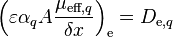 and
and 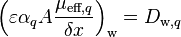 and modifying the central coefficient slightly, since
  and
and  , Equation 11 reduces to
-
(12)
![= \left[\text{max}\left(-F_{\text{e},q},0\right) + D_{\text{e},q} + \text{max}\left(F_{\text{w},q},0\right) + D_{\text{w},q} + \left(F_{\text{e},q} - F_{\text{w},q}\right)\right]u_{\text{P},q}](/kraken/images/math/6/a/1/6a14c9996a6210d0e6cd00faf571de77.png)
![-\left[\text{max}\left(-F_{\text{e},q},0\right) + D_{\text{e},q}\right]u_{\text{E},q} - \left[\text{max}\left(F_{\text{w},q},0\right) + D_{\text{w},q}\right]u_{\text{W},q}](/kraken/images/math/8/4/5/845bc7a2f0606db36b351968e43f48dc.png)
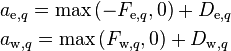
Identifying the coefficients of neighboring velocities
-

(13)
-

(14)
leads to a general form
-
(15)
![= \left[a_{\text{e},q} + a_{\text{w},q} + \left(F_{\text{e},q} - F_{\text{w},q}\right)\right]u_{\text{P},q} - a_{\text{e},q}u_{\text{E},q} - a_{\text{w},q}u_{\text{W},q}](/kraken/images/math/9/f/1/9f18c89b7e860a7008e2c3c14d212be7.png)
Substituting the results of Equation 15 into Equation 7 and continuing with the development
-
![\Rightarrow\left[a_{\text{e},q} + a_{\text{w},q} + \left(F_{\text{e},q} - F_{\text{w},q}\right)\right]u_{\text{P},q} - a_{\text{e},q}u_{\text{E},q} - a_{\text{w},q}u_{\text{W},q}](/kraken/images/math/a/1/f/a1fa90c3136e1fb0a88bb43780b8e057.png)
(16)
![= \left[\text{max}\left(\Gamma_{pq},0\right)u_p - \text{max}\left(-\Gamma_{pq},0\right)u_q\right] - \varepsilon \alpha_q V \nabla p + \varepsilon \alpha_q \rho_q V g](/kraken/images/math/6/e/6/6e6339c3a814a64f32d7fbae576cd0f5.png)

At this point, the conservation of mass equation times cell velocity,  , is subtracted from Equation 16
-
![\Rightarrow\left[a_{\text{e},q} + a_{\text{w},q} + \left(F_{\text{e},q} - F_{\text{w},q}\right) - \left(F_{\text{e},q} - F_{\text{w},q}\right)\right]u_{\text{P},q} - a_{\text{e},q}u_{\text{E},q} - a_{\text{w},q}u_{\text{W},q}](/kraken/images/math/d/a/2/da2a247d8ef6a063d9411ae2a21910f1.png)
(17)
![= \left[\text{max}\left(\Gamma_{pq},0\right)u_p - \text{max}\left(-\Gamma_{pq},0\right)u_q\right] - \left(\Gamma_{pq} + S_{\text{mass},q}\right)u_{\text{P},q}](/kraken/images/math/3/b/5/3b5b23c7e405935814c27671016cf3c7.png)
Splitting the mass source term
-
![\Leftrightarrow\left[a_{\text{e},q} + a_{\text{w},q}\right]u_{\text{P},q} - a_{\text{e},q}u_{\text{E},q} - a_{\text{w},q}u_{\text{W},q}](/kraken/images/math/7/9/8/798ff496cdad3f190128786f0082a3d4.png)
(18)
![= \left[\text{max}\left(\Gamma_{pq},0\right)u_{\text{P},p} - \text{max}\left(-\Gamma_{pq},0\right)u_{\text{P},q}\right]](/kraken/images/math/8/8/8/888e32a31eaccebdb6e64f843664cf73.png)
![-\left[\text{max}\left(\Gamma_{pq},0\right) - \text{max}\left(-\Gamma_{pq},0\right) + \text{max}\left(S_{\text{mass},q},0\right) - \text{max}\left(-S_{\text{mass},q},0\right)\right]u_{\text{P},q}](/kraken/images/math/7/2/7/72744f41c842afd2c31892b167d36043.png)
-
![\Leftrightarrow\left[a_{\text{e},q} + a_{\text{w},q} + \text{max}\left(\Gamma_{pq},0\right) + \text{max}\left(S_{\text{mass},q},0\right) + \text{max}\left(-\Gamma_{pq},0\right)\right]u_{\text{P},q} - a_{\text{e},q}u_{\text{E},q} - a_{\text{w},q}u_{\text{W},q}](/kraken/images/math/9/d/4/9d4c1ac8d4b129ea8c226ede11042aaa.png)
(19)
![= \left[\text{max}\left(-\Gamma_{pq},0\right) + \text{max}\left(-S_{\text{mass},q},0\right)\right]u_q + \text{max}\left(\Gamma_{pq},0\right)u_p](/kraken/images/math/4/c/8/4c836d593aa8f252d8c50cdf3a143b27.png)
Since the right-hand side contains only references to the central cell, subscripts P have been dropped from right-hand side to simplify the notation. Note that the diagonal element of the coefficient matrix contains the split terms,  , resulting from the subtraction of the mass equation times cell velocity, while the counterparts,
 ![\left[\text{max}\left(-\Gamma_{pq},0\right) + \text{max}\left(-S_{\text{mass},q},0\right)\right]u_q](/kraken/images/math/f/e/a/fea79e1112ad0a4cdd9ecaaae42e9492.png) , remain on the right-hand side. These are not considered as momentum source terms, as such, since they are only artifacts of the derivation procedure.
, remain on the right-hand side. These are not considered as momentum source terms, as such, since they are only artifacts of the derivation procedure.
In preparation for casting Equation 19 into a vector form over the phases, a phase coupling matrix,  , is formed
-
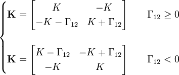
(20)
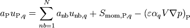
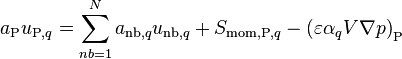
Finally, denoting the central coefficient by  and casting Equation 19 into a vector form (over the phases) the final form, in which the equations are actually solved, is obtained. For simplicity’s sake, the equation is written only for the first 3 cells (c1, c2 and c3).
-
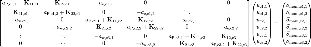
(21)
where:
![S_{\text{mom},\text{c1},q} = \Big[ \text{max}\left(-S_{\text{mass},q},0\right)u_q -\varepsilon \alpha_q V \nabla p + \varepsilon \alpha_q \rho_q V g - \tfrac{1}{2} \varepsilon^3 \alpha_q \rho_q C V \left| u_q \right| u_q + S_{\text{mom},q} \Big]_{\text{c1}}](/kraken/images/math/b/e/f/bef1f8fbfe9caf25178751a207d1a49d.png)
and
-
volume fraction of phase q [-],
volumetric mass transfer rate from phase p to q [kg/m3s],
mass transfer rate from phase p to q [kg/s], 
distance between two adjacent cell centers [m],
porosity, fluid fraction of cell volume [-], 
effective viscosity of phase q [Ns/m2],
density of phase q [kg/m3],
face area [m2], 
inertial loss coefficient [1/m],
face mass flow rate [kg/s], 
acceleration of gravity [m/s2], 
volumetric interphase drag coefficient [kg/m3s], 
interphase drag coefficient [kg/s],
face normal pointing out of the cell (1 for east face, -1 for west face), 
pressure [Pa],
volumetric mass source to phase q [kg/m3s],
mass source to phase q [kg/s], 
volumetric momentum source to phase q [N/m3], 
momentum source to phase q [N],
velocity of phase q [m/s], 
cell volume [m3], subscript c1 refers to first cell, subscript c2 refers to second cell, subscript c3 refers to third cell, subscript e east face (the face in the negative x-direction), subscript E east neighbor (the cell in the negative x-direction), subscript w west face (the face in the positive x-direction), subscript W west neighbor (the cell in the positive x-direction), subscript P central cell (the cell for which the equation is written), subscript q current phase for which the equation is written (1 = primary, 2 = secondary), subscript p the other phase (p = 2 for q = 1 and p = 1 for q = 2), subscript pq indicates exchange between phases (e.g. mass transfer from phase p to q).
Conservation of Total Enthalpy

Conservation of total enthalpy (of phase q) can be written as
-
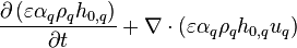
(22)
![= \nabla\cdot\left(\varepsilon \alpha_q \lambda_{\text{eff},q} \nabla T_q \right) + \left[\text{max}\left(\gamma_{pq},0\right) h_{0,\text{cre}} - \text{max}\left(-\gamma_{pq},0\right) h_{0,\text{des}}\right]](/kraken/images/math/f/d/d/fdd7504ef94955b652efccf6553d3a0e.png)
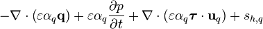
Disregarding the transient terms and moving the diffusion term to the left-hand side leads to
-

(23)
![= \left[\text{max}\left(\gamma_{pq},0\right) h_{0,\text{cre}} - \text{max}\left(-\gamma_{pq},0\right) h_{0,\text{des}}\right] - \nabla\cdot\left(\varepsilon \alpha_q \mathbf{q} \right) + \nabla\cdot\left(\varepsilon \alpha_q \boldsymbol{\tau} \cdot \mathbf{u}_q \right) + s_{h,q}](/kraken/images/math/a/5/7/a57e9b9ee32ff5d733461f3580589d60.png)
Total enthalpy is defined as the sum of specific enthalpy, kinetic energy and potential energy
-
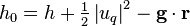
(24)
where  is the dot product of gravity vector,
  , and location vector,
  , a vector pointing from the reference level to the evaluated location. The total enthalpies related to phase change can be defined as
-
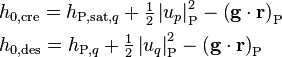
(25)
In other words, when mass is transferred to phase q (“created”), it brings with it the saturation enthalpy of phase q,  , and the kinetic energy of phase p,
  . When mass is transferred from phase q (“destroyed”), it leaves with the enthalpy and kinetic energy of phase q,
 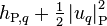 . It is chosen that the potential energy associated with phase change is evaluated at the center of the cell,
  .
.
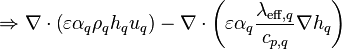
Substituting Equation 24 and Equation 25 to Equation 23 and rearranging terms
-

(26)
![= \left[\text{max}\left(\gamma_{pq},0\right) \left(h_{\text{P,sat,}q} + \tfrac{1}{2} \left| u_p \right|^2_{\text{P}} - \left(\mathbf{g} \cdot \mathbf{r}\right)_{\text{P}}\right) - \text{max}\left(-\gamma_{pq},0\right) \left(h_{\text{P,}q} + \tfrac{1}{2} \left| u_q \right|^2_{\text{P}} - \left(\mathbf{g} \cdot \mathbf{r}\right)_{\text{P}}
\right)\right]](/kraken/images/math/4/6/f/46fe563fa8f9fd8a50836ed1e5d01adb.png)

At this point, an approximation is introduced: the diffusion term is expressed relative to the gradient of enthalpy, instead of temperature, as follows. This approximation is considered to be sufficiently accurate for small enthalpy differences.
-
(27)
Equation 27 is discretized for an interior cell, shown in Figure 3, by volume integration over cell P.
-
![\Leftrightarrow \iiint\limits_V \left[\nabla\cdot\left(\varepsilon \alpha_q \rho_q h_q u_q\right) - \nabla\cdot\left(\varepsilon \alpha_q \frac{\lambda_{\text{eff},q}}{c_{p,q}} \nabla h_q \right)\right]\, \text{d}V](/kraken/images/math/c/4/c/c4c9388c682095dff08e5411a06cda7d.png)
(28)
![= \iiint\limits_V \Big\{ \left[\text{max}\left(\gamma_{pq},0\right) \left(h_{\text{P,sat,}q} + \tfrac{1}{2} \left| u_p \right|^2_{\text{P}} - \left(\mathbf{g} \cdot \mathbf{r}\right)_{\text{P}}\right) - \text{max}\left(-\gamma_{pq},0\right) \left(h_{\text{P,}q} + \tfrac{1}{2} \left| u_q \right|^2_{\text{P}} - \left(\mathbf{g} \cdot \mathbf{r}\right)_{\text{P}}\right)\right]](/kraken/images/math/0/2/d/02d773d05b3277198585d15573db3e39.png)

As with the conservation of mass and momentum above, the divergence terms on the left-hand side of the equation are transformed into surface integrals over the cell faces using the divergence theorem.
-
![\Leftrightarrow \iint\limits_{A}\!\!\!\!\!\!\!\!\!\!\!\subset\!\supset \left[\left(\varepsilon \alpha_q \rho_q h_q u_q\right)\cdot n - \left(\varepsilon \alpha_q \frac{\lambda_{\text{eff},q}}{c_{p,q}} \frac{\Delta h_q}{\delta x}\right)\cdot n\right]\, \text{d}A](/kraken/images/math/3/7/5/375c2548500811666e354b0c6064648b.png)
(29)
Developing the left-hand side first.
-
(30)


Adopting upwind discretization for the enthalpy fluxes on the cell faces
-
(31)
and rearranging terms
-
(32)
![= \left[ \text{max}\left(F_{\text{e},q},0\right) + \text{max}\left(-F_{\text{w},q},0\right) + \left(\varepsilon \alpha_q A \frac{\lambda_{\text{eff},q}}{c_{p,q}\delta x}\right)_{\text{e}} + \left(\varepsilon \alpha_q A \frac{\lambda_{\text{eff},q}}{c_{p,q}\delta x}\right)_{\text{w}} \right] h_{\text{P},q}](/kraken/images/math/b/7/c/b7cd5ddaf5739424a772224ad76c435d.png)
![- \left[ \text{max}\left(-F_{\text{e},q},0\right) + \left(\varepsilon \alpha_q A \frac{\lambda_{\text{eff},q}}{c_{p,q}\delta x}\right)_{\text{e}} \right] h_{\text{E},q} - \left[ \text{max}\left(F_{\text{w},q},0\right) + \left(\varepsilon \alpha_q A \frac{\lambda_{\text{eff},q}}{c_{p,q}\delta x}\right)_{\text{w}} \right] h_{\text{W},q}](/kraken/images/math/5/6/3/563ccf430a94c716f3f2bea92515becf.png)
Denoting 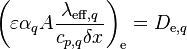 and
and 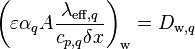 and modifying the central coefficient slightly, since and , Equation 32 reduces to
-
(33)
![= \left[ \text{max}\left(-F_{\text{e},q},0\right) + D_{\text{e},q} + \text{max}\left(F_{\text{w},q},0\right) + D_{\text{w},q} + \left( F_{\text{e},q} - F_{\text{w},q} \right) \right] h_{\text{P},q}](/kraken/images/math/e/2/b/e2bce9cdc7a6b6f9761cdb2da5370d22.png)
![- \left[ \text{max}\left(-F_{\text{e},q},0\right) + D_{\text{e},q} \right] h_{\text{E},q}
- \left[ \text{max}\left(F_{\text{w},q},0\right) + D_{\text{w},q} \right] h_{\text{W},q}](/kraken/images/math/7/a/8/7a8ff932eeb0976faa4491f20159b29e.png)
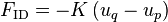
Identifying the coefficients of neighboring velocities as
-
(34)
leads to a general form
-
(35)
![= \left[ a_{\text{e},q} + a_{\text{w},q} + \left( F_{\text{e},q} - F_{\text{w},q} \right) \right] h_{\text{P},q} - a_{\text{e},q} h_{\text{E},q} - a_{\text{w},q} h_{\text{W},q}](/kraken/images/math/7/f/3/7f3d736f0dc96567420cd56623265fb4.png)
Substituting the results of Equation 35 into Equation 29 and continuing with the development
-
![\Rightarrow \left[ a_{\text{e},q} + a_{\text{w},q} + \left( F_{\text{e},q} - F_{\text{w},q} \right) \right] h_{\text{P},q} - a_{\text{e},q} h_{\text{E},q} - a_{\text{w},q} h_{\text{W},q}](/kraken/images/math/d/2/9/d29ac63c53bbff20a9fd593d46fba42a.png)
(36)
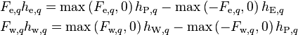
Integrating the right-hand side term by term. The phase change term reduces to
-
![\iiint\limits_V \left[\text{max}\left(\gamma_{pq},0\right) \left(h_{\text{P,sat,}q} + \tfrac{1}{2} \left| u_p \right|^2_{\text{P}} - \left(\mathbf{g} \cdot \mathbf{r}\right)_{\text{P}}\right) - \text{max}\left(-\gamma_{pq},0\right) \left(h_{\text{P,}q} + \tfrac{1}{2} \left| u_q \right|^2_{\text{P}} - \left(\mathbf{g} \cdot \mathbf{r}\right)_{\text{P}}\right)\right] \text{d}V](/kraken/images/math/9/4/d/94d16fe4814cbbc0b38a07f979da7f9d.png)
(37)
![= \left[\text{max}\left(\Gamma_{pq},0\right) \left(h_{\text{P,sat,}q} + \tfrac{1}{2} \left| u_p \right|^2_{\text{P}} - \left(\mathbf{g} \cdot \mathbf{r}\right)_{\text{P}}\right) - \text{max}\left(-\Gamma_{pq},0\right) \left(h_{\text{P,}q} + \tfrac{1}{2} \left| u_q \right|^2_{\text{P}} - \left(\mathbf{g} \cdot \mathbf{r}\right)_{\text{P}}\right)\right]](/kraken/images/math/3/d/5/3d5e238b6b16cc5bef8146947459d126.png)
The divergence terms,  , are handled equivalently to the divergence terms on the left-hand side of the equation
-
![\iiint\limits_V \left[ -\nabla\cdot\left(\tfrac{1}{2}\varepsilon \alpha_q \rho_q \left| u_q \right|^2 u_q\right)+\nabla\cdot\left(\varepsilon \alpha_q \rho_q \left( \mathbf{g} \cdot \mathbf{r} \right)u_q\right)\right] \text{d}V](/kraken/images/math/0/0/a/00a13852e8dc45a851e054d01dbf4dec.png)
(38)
![= -\tfrac{1}{2}\left( F_{\text{e},q} \left| u_q \right|^2_{\text{e}} - F_{\text{w},q} \left| u_q \right|^2_{\text{w}}\right)
+ \left[ F_{\text{e},q} \left( \mathbf{g} \cdot \mathbf{r} \right)_{\text{e}} - F_{\text{w},q} \left( \mathbf{g} \cdot \mathbf{r} \right)_{\text{w}}\right]](/kraken/images/math/7/4/f/74f8a00fd2f9963415d0f6a157798bae.png)
Heat source due to heat fluxes at the cell faces,  , are dropped out. Heat sources from an external source, such as neutronics solver, will be implemented later.
Friction work is replaced with the following simplified formulation
-
![\iiint\limits_V \left[\nabla\cdot\left(\varepsilon \alpha_q \boldsymbol{\tau} \cdot \mathbf{u}_q \right) \right] \text{d}V
= \left( F_{\text{D}} + F_{\text{ID}} \right) u_{\text{P},q}](/kraken/images/math/2/8/3/2831c23f4252dfeaaeb58343e701866a.png)
(39)
where the drag force,  , and the interfacial drag force,
  , are calculated from the following relations
-
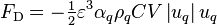
(40)
-
(41)
Volume integral of volumetric enthalpy source to phase q is simply
-
(42)
Combining equations Equation 36, Equation 37, Equation 38, Equation 39 and Equation 42 leads to
-
(43)
![-\tfrac{1}{2}\left( F_{\text{e},q} \left| u_q \right|^2_{\text{e}} - F_{\text{w},q} \left| u_q \right|^2_{\text{w}}\right)
+ \left[ F_{\text{e},q} \left( \mathbf{g} \cdot \mathbf{r} \right)_{\text{e}} - F_{\text{w},q} \left( \mathbf{g} \cdot \mathbf{r} \right)_{\text{w}}\right] + \left( F_{\text{D}} + F_{\text{ID}} \right) u_{\text{P},q} + S_{h,q}](/kraken/images/math/5/9/5/5954bac5901404f5913a778213ec78a7.png)
Rearranging terms
-
![\Leftrightarrow \left[ a_{\text{e},q} + a_{\text{w},q} + \left( F_{\text{e},q} - F_{\text{w},q} \right) \right] h_{\text{P},q} - a_{\text{e},q} h_{\text{E},q} - a_{\text{w},q} h_{\text{W},q}](/kraken/images/math/0/3/c/03cc4b0a973851e349f9b7c78be33ed2.png)
(44)
![= -\tfrac{1}{2} \left[ F_{\text{e},q} \left| u_q \right|^2_{\text{e}} - F_{\text{w},q} \left| u_q \right|^2_{\text{w}} + \text{max}\left(-\Gamma_{pq},0\right) \left| u_q \right|^2_{\text{P}} - \text{max}\left(\Gamma_{pq},0\right) \left| u_p \right|^2_{\text{P}} \right]](/kraken/images/math/5/1/a/51a31a98f477e60753bda77475d65764.png)
![+ \left[ F_{\text{e},q} \left(\mathbf{g} \cdot \mathbf{r}\right)_{\text{e}} - F_{\text{w},q} \left(\mathbf{g} \cdot \mathbf{r}\right)_{\text{w}} - \Gamma_{pq} \left(\mathbf{g} \cdot \mathbf{r}\right)_{\text{P}} \right] + \left[ \text{max}\left(\Gamma_{pq},0\right) h_{\text{P,sat,}q} - \text{max}\left(-\Gamma_{pq},0\right) h_{\text{P},q}\right]](/kraken/images/math/a/4/b/a4baf85c452f169542e3a557f7421f6e.png)
At this point, the conservation of mass equation times cell specific enthalpy,  , is subtracted from Equation 44
-
![\Rightarrow \left[ a_{\text{e},q} + a_{\text{w},q} + \left( F_{\text{e},q} - F_{\text{w},q} \right) - \left( F_{\text{e},q} - F_{\text{w},q} \right) \right] h_{\text{P},q} - a_{\text{e},q} h_{\text{E},q} - a_{\text{w},q} h_{\text{W},q}](/kraken/images/math/0/6/9/0692f516d0b9ba58ef462716ce31695d.png)
(45)

Splitting the mass source terms into negative and positive parts
-
![\Leftrightarrow \left[ a_{\text{e},q} + a_{\text{w},q} + \left( F_{\text{e},q} - F_{\text{w},q} \right) - \left( F_{\text{e},q} - F_{\text{w},q} \right) \right] h_{\text{P},q} - a_{\text{e},q} h_{\text{E},q} - a_{\text{w},q} h_{\text{W},q}](/kraken/images/math/d/e/f/def5f2043b64c02949ecfd9d92c3e4fc.png)
(46)
![+ \left( F_{\text{D}} + F_{\text{ID}} \right) u_{\text{P},q} + S_{h,q} - \left[ \text{max}\left(\Gamma_{pq},0\right) - \text{max}\left(-\Gamma_{pq},0\right) \right] h_{\text{P},q} - \left[ \text{max}\left(S_{\text{mass},q},0\right) - \text{max}\left(-S_{\text{mass},q},0\right)\right] h_{\text{P},q}](/kraken/images/math/a/6/5/a65b3f9cfc141ed5dba113645b11ffed.png)
and rearranging the terms leads to the final form
-
![\Leftrightarrow \left[ a_{\text{e},q} + a_{\text{w},q} + \text{max}\left(\Gamma_{pq},0\right) + \text{max}\left(S_{\text{mass},q},0\right) + \text{max}\left(-\Gamma_{pq},0\right) \right] h_{\text{P},q} - a_{\text{e},q} h_{\text{E},q} - a_{\text{w},q} h_{\text{W},q}](/kraken/images/math/3/3/9/339b65a52e91975d2bb2b98e524e992a.png)
(47)
![= \left[ \text{max}\left(-\Gamma_{pq},0\right) + \text{max}\left(-S_{\text{mass},q},0\right) \right] h_{\text{P},q} + \text{max}\left(\Gamma_{pq},0\right) h_{\text{P,sat},q}](/kraken/images/math/1/c/6/1c656140e4ff7956c65b6852c003c96c.png)
![- \tfrac{1}{2} \left[ F_{\text{e},q} \left| u_q \right|^2_{\text{e}} - F_{\text{w},q} \left| u_q \right|^2_{\text{w}} + \text{max}\left(-\Gamma_{pq},0\right) \left| u_q \right|^2_{\text{P}} - \text{max}\left(\Gamma_{pq},0\right) \left| u_p \right|^2_{\text{P}} \right]](/kraken/images/math/f/3/5/f359d9f7f4704354f76d242238e54309.png)
![+ \left[ F_{\text{e},q} \left(\mathbf{g} \cdot \mathbf{r}\right)_{\text{e}} - F_{\text{w},q} \left(\mathbf{g} \cdot \mathbf{r}\right)_{\text{w}} - \Gamma_{pq} \left(\mathbf{g} \cdot \mathbf{r}\right)_{\text{P}} \right] + \left( F_{\text{D}} + F_{\text{ID}} \right) u_{\text{P},q} + S_{h,q}](/kraken/images/math/9/f/f/9ffcca7209087a4a6128af8645cfdaae.png)
where:
-
volume fraction of phase q [-],
volumetric mass transfer rate from phase p to q [kg/m3s],
mass transfer rate from phase p to q [kg/s],
distance between two adjacent cell centers [m],
porosity, fluid fraction of cell volume [-], 
effective thermal conductivity of phase q [W/mK],
density of phase q [kg/m3],
face area [m2],
inertial loss coefficient [1/m],
face mass flow rate [kg/s],
drag force [N],
interfacial drag force [N],
acceleration of gravity (vector) [m/s2], 
specific enthalpy of phase q [J/kg], 
total enthalpy of phase q [J/kg],
interphase drag coefficient [kg/s],
face normal pointing out of the cell (1 for east face, -1 for west face),
pressure [Pa],
location vector [m], 
volumetric energy source to phase q [W/m3], 
energy source to phase q [W],
volumetric mass source to phase q [kg/m3s],
mass source to phase q [kg/s],
velocity of phase q [m/s],
cell volume [m3], subscript c1 refers to first cell, subscript c2 refers to second cell, subscript c3 refers to third cell, subscript e east face (the face in the negative x-direction), subscript E east neighbor (the cell in the negative x-direction), subscript w west face (the face in the positive x-direction), subscript W west neighbor (the cell in the positive x-direction), subscript P central cell (the cell for which the equation is written), subscript q current phase for which the equation is written (1 = primary, 2 = secondary), subscript p the other phase (p = 2 for q = 1 and p = 1 for q = 2), subscript pq indicates exchange between phases (e.g. mass transfer from phase p to q).
Same as the conservation of momentum equations above, Equation 47 is solved in a phase-coupled manner, even though, due to the chosen interphase heat and mass transfer concept, the phase coupling coefficients are zero. As a reminder, the terms ![\left[ \text{max}\left(\Gamma_{pq},0\right) + \text{max}\left(S_{\text{mass},q},0\right) \right] h_{\text{P},q}](/kraken/images/math/1/c/9/1c9f38e180a3db348cdfc05ae9147fa5.png) on the left-hand side and
on the left-hand side and ![\left[ \text{max}\left(-\Gamma_{pq},0\right) + \text{max}\left(-S_{\text{mass},q},0\right) \right] h_{\text{P},q}](/kraken/images/math/5/4/e/54e58344b20183faeacb94d3bfec8f88.png) on the right-hand side result from the derivation procedure and are not considered as source terms. The terms
on the right-hand side result from the derivation procedure and are not considered as source terms. The terms  on the left-hand side and
  on the right-hand side constitute the enthalpy source due to phase change. Note, however, that in the event of mass transfer from phase q, the terms on both sides of the equation cancel out.
Face Velocity Equation
The basic intent here is to find a relation for the face velocities,  , that depend on the momentum solution of the adjacent cells and the pressure difference over the face in question. The importance of this formulation is paramount, for it determines whether a solution that satisfies continuity can coexist with a monotonous velocity field or not.
The first attempts at a solution algorithm based on a collocated formulation (both pressures and velocities are stored at cell centers) were found to produce highly oscillatory pressure and velocity fields. One of the first, or at least the most widely known, remedies, the Pressure Weighted Interpolation Method (PWIM), was proposed by Rhie and Chow [1] for single-phase flow. It quickly gained popularity in combination with the SIMPLE[2] based methods. The original form of PWIM, however, is not without problems and several authors have since suggested modifications to it. The under-relaxation and time-step dependencies were first reported by Majumdar[3] and Choi[4], respectively. Recently, a well-written article was introduced by Pascau[5], which includes a thorough and elegant derivation for the face velocity equation that deals with both the under-relaxation and time-step dependencies. In addition, the possible choices made in the interpolation of the terms in the face velocity equations and the different methods that result are well illustrated.[5]
In the following, the derivation by Pascau[5] is presented and slightly expanded for phase q. Although not directly evident, the resulting form is under-relaxation factor independent.
Starting from a compacted form of Equation 19, where all the other source terms, except the pressure gradient, are included in  .
.
-
(48)
Under-relax
-

(49)
Multiply by 
-

(50)
Divide by 
-

(51)
Writing a fictional momentum equation for face f that is identical in form to Equation 51
-

(52)
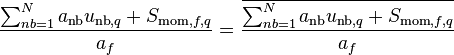
and for momentum interpolated over face f
-

(53)
Pressure Weighted Interpolation Method (PWIM):
-
(54)
Solving 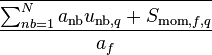 from Equation 53 and substituting it to Equation 52 leads to:
-
![u_{f,q} = \overline{u_{f,q}} + \alpha_u \left[ \frac{\overline{\left( \varepsilon \alpha_q V \nabla p \right)_f}} {a_f} - \frac{\left( \varepsilon \alpha_q V \nabla p \right)_f} {a_f} \right] + \left( 1 - \alpha_u \right) \left( u_{f,q}^* - \overline{u_{f,q}^*} \right)](/kraken/images/math/e/a/c/eacabd967882ebe144f1117b83d38241.png)
(55)
Phase-Coupled Face Velocity Equation
In this section, a phase-coupled version of the face velocity equations is developed. Similar ideas have been previously employed by Kunz et al. [6] and Vasquez and Ivanov [7]. Starting from a compacted form of Equation 19, where all the other source terms, except the pressure gradient, are included in .
-
(56)
Under-relaxing the equation, as it has already been done in the solution of momentum equations in the previous step of the solution algorithm ( = velocity under-relaxation factor).  denotes the value of at the previous iteration.
-

(57)
Multiply by
-

(58)
Casting Equation 58 into a vector form (over phases)
-

(59)
Denoting 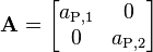 ,
, 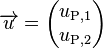 ,
,  , and
, and 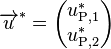 to simplify the notation.
-

(60)
Separating a part of the interphase friction from the source term
-

(61)
and denoting 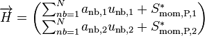 , and
, and 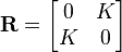 .
.
-

(62)
Subtracting  from both sides of the equation.
-

(63)
Since  is not available on the right-hand side, it is replaced by
  .
.
-

(64)
Multiplying both sides by 
-

(65)
Writing a fictitious momentum equation for face f that is identical in form to Equation 65
-

(66)
and for momentum interpolated over face f
-

(67)
When adopting the Pressure Weighted Interpolation Method (PWIM), the approach originally used by Rhie and Chow [1] can be interpreted as an interpolation of 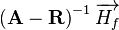 and
and  over the face:
-

(68)
Solving  from Equation 67 and substituting it to Equation 66 leads to
-
![\Rightarrow \overrightarrow{u_f} = \overline{\overrightarrow{u_f}}
+ \alpha_u \left[\overline{\left( \varepsilon V \nabla p \right)_{f} \left( \mathbf{A} - \mathbf{R} \right)^{-1} \overrightarrow{\alpha_f}} - \left( \varepsilon V \nabla p \right)_{f} \left( \mathbf{A} - \mathbf{R} \right)^{-1} \overrightarrow{\alpha_f} \right]
+ \left( 1 - \alpha_u \right) \left( \overrightarrow{u_f}^* - \overline{\overrightarrow{u_f}^*} \right)](/kraken/images/math/4/4/8/448497c7d66a133a705ae93428e83afc.png)
(69)
Rearranging variables and using 
-
![\Rightarrow \overrightarrow{u_f} = \overline{\overrightarrow{u_f}}
+ \alpha_u \left[\overline{\left( \varepsilon V \right)_{f} \left( \mathbf{A} - \mathbf{R} \right)^{-1} \overrightarrow{\alpha_f} \nabla p_f} - \overline{\left( \varepsilon V \right)_{f} \left( \mathbf{A} - \mathbf{R} \right)^{-1} \overrightarrow{\alpha_f}} \nabla p_f \right]
+ \left( 1 - \alpha_u \right) \left( \overrightarrow{u_f}^* - \overline{\overrightarrow{u_f}^*} \right)](/kraken/images/math/1/a/0/1a04641cfbd14321236ad5c9803d1fbb.png)
(70)
Computation of face velocity involves the solution of two systems of equations for each face
-
(71)
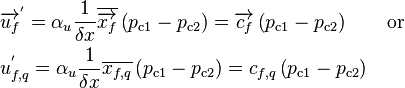
Linear interpolation of the first term inside the brackets, in Equation 70, yields
-

(72)
and the second term reduces to
-
![\overline{\left( \varepsilon V \right)_{f} \left( \mathbf{A} - \mathbf{R} \right)^{-1} \overrightarrow{\alpha_f}} \nabla p_f = \left[ \beta \overrightarrow{x_{\text{c1}}} + \left( 1 - \beta \right) \overrightarrow{x_{\text{c2}}} \right] \frac{p_{\text{c2}} - p_{\text{c1}}}{\delta x} = \frac{1}{\delta x} \overline{\overrightarrow{x_f}} \left( p_{\text{c2}} - p_{\text{c1}} \right)](/kraken/images/math/4/3/5/43560e52915a14b00d7b5ecef5b54de9.png)
(73)
Substituting the results of Equation 72 and Equation 73 to Equation 70 leads to the final form, in which the equation is implemented in the code:
-
![\Rightarrow \overrightarrow{u_f} = \overline{\overrightarrow{u_f}}
+ \alpha_u \left[\overline{\overrightarrow{x_f} \nabla p_f} - \frac{1}{\delta x} \overline{\overrightarrow{x_f}} \left( p_{\text{c2}} - p_{\text{c1}} \right) \right]
+ \left( 1 - \alpha_u \right) \left( \overrightarrow{u_f}^* - \overline{\overrightarrow{u_f}^*} \right)](/kraken/images/math/8/8/7/887efe58a11959512a22035d4e8ce2ae.png)
(74)
Pressure & Volume Fraction Correction
The pressure & volume fraction correction method (pα-correction) starts with the idea of developing such corrections to pressure  , phase volume fraction
  , and in the process, to face mass flow rates
-
(75)
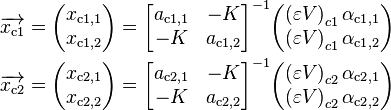
that continuity of both phases (and consequently the sum of phases) is satisfied at the end of the iteration:
-
(76)
Starred values represent the latest available values and the dotted values stand for the corrections. The sum of volume fraction corrections is zero, which for a two-phase system means that  .
.
Face mass flow rates are functions of both velocity and volume fraction evaluated at the face. To obtain the influence of both pressure correction (through changes in face velocity) and volume fraction correction on face mass flow rate, face mass flow rate is derivated with respect to velocity and volume fraction.
-
![\begin{align}
F_{f,q}^' &= D \left( F_{f,q} \right) = D \left( \varepsilon \alpha_q \rho_q u_q A \right)_f = \left( \varepsilon \rho_q A \right)_f \left[ D \left( \alpha_q u_q^' \right)_f + D \left( \alpha_q^' u_q \right)_f \right] \\
&= \left( \varepsilon \alpha_q \rho_q A \right)_f u_{f,q}^' + \left( \varepsilon \rho_q u_{q} A \right)_f \alpha_{f,q}^'
\end{align}](/kraken/images/math/2/8/5/285d81f7141f7ee6aaf64ca9540893de.png)
(77)
The relation between pressure and velocity corrections is obtained from equation Equation 74 by replacing the pressures of the adjacent cells by the corresponding pressure corrections and disregarding all the other terms. Note that the pressure difference,  , has been reversed to produce positive pressure coefficients,
  .
.
-
(78)
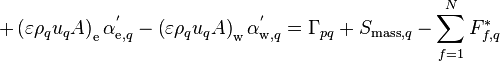
The development of the method begins with the phase continuity equations.
-
(79)
Introducing the corrected face mass flow rates from Equation 75 into Equation 79.
-

(80)
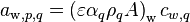
Writing the face mass flow corrections, , with the help of derivatives developed in Equation 77.
-

(81)
Substituting Equation 78 into Equation 81 to express the velocity correction in terms of adjacent pressure corrections.
-

(82)
Denoting 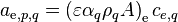 ,
,  , and
, and 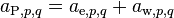 to simplify the notation:
-

(83)
Upwind discretization is adopted for the remaining face values on the left-hand side:
-

(84)
Denoting  ,
,  , and
, and  and substituting the upwinded terms to Equation 83
-
(85)
Writing Equation 85 for both phases and substituting to the primary phase equation leads to the final form:
-

(86)
A single system of equations is formed from Equation 86 by stacking up the primary phase equations on top of the secondary phase equations. Pressure correction is chosen as the unknown for the primary phase equations and secondary phase volume fraction correction as the unknown for the secondary phase equations. The resulting system of equations (for a 1D channel consisting of three adjacent cells) is shown below.
-
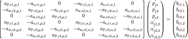
(87)
For some linear solvers it might be beneficial to load the equations in a different order. The ordering shown in Equation 21 for the coupled momentum equations produces a significant reduction in bandwidth for large systems of equations, but for such a small number of cells (~20 cells in a single channel) the efficiency gain is probably insignificant.
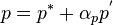
After the solution of Equation 87 face velocities are corrected with
-
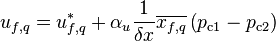
(88)
phase volume fractions are corrected with
-
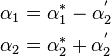
(89)
and pressure is corrected with
-
(90)
Note that the pressure correction can be under-relaxed, with an under-relaxation factor  , while the full amount of the correction needs to be applied to the face velocities and volume fractions in order to produce face mass flow rates that satisfy continuity. Cell-centered velocities can still be under-relaxed in the usual manner when solving the momentum equations, since under-relaxation has been taken into account in the face velocity equations and the pressure & volume fraction correction equations.
Solution Algorithm
The numerical solution of the governing equations relies on a pressure-based segregated approach, which means that pressure has been selected as one of the solution variables, instead of density, and each solution variable is solved from its own system of equations, one after the other. The only exception, which moves the classification of the solution method towards coupled methods, is that pressure and volume fraction corrections are solved together from a single system of equations.
The implemented solution algorithm belongs to the SIMPLE family of algorithms, extended to multiphase flow from the original single-phase SIMPLE algorithm of Patankar[2], and bears close resemblance to both the Coupled Phasic Exchange algorithm of Kunz et al. [6] and the Phase Coupled SIMPLE algorithm of Vasquez and Ivanov [7]. A schematic of the solution algorithm is shown in Figure 4.
Momentum Transfer
The forces that drive the fluid flow are placed on the right-hand side of the momentum conservation equations, best seen in Equation 16 before the linearization and other modifications. These are called the momentum source terms and they include the effects caused by phase change, pressure gradient, gravitational forces, pressure loss caused by the porous material, interfacial friction, and possibly user-defined momentum sources:
-
![S = \left[\text{max}\left(\Gamma_{pq},0\right)u_p - \text{max}\left(-\Gamma_{pq},0\right)u_q\right] - \varepsilon \alpha_q V \nabla p + \varepsilon \alpha_q \rho_q V g
- \tfrac{1}{2} \varepsilon^3 \alpha_q \rho_q C V \left| u_q \right| u_q - K\left(u_q - u_p\right) + S_{\text{mom},q}](/kraken/images/math/1/5/e/15efe1bae2a919baffd687cf1f475962.png)
(91)
At this point a parameter fundamental to internal flows is introduced, since it often appears in 1D pressure drop correlations. Hydraulic diameter  [m] is defined in terms of either the flow area,
  [m2], and wetted perimeter,
  [m], or the fluid volume,
  [m3], and wetted surface area,
  [m2], as follows
-
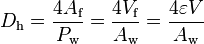
(92)
where fluid volume, [m3], can be expressed as the product of total volume, [m3], and porosity, [-].
Pressure loss
The solid structures inside the flow channel exert a force that resists the fluid flow. The pressure loss (or drag) is modelled as an inertial resistance:
-
(93)
The inertial loss coefficient, [1/m], is defined as the ratio of the moody friction factor to hydraulic diameter:
-

(94)
The friction factor,  [-], depends on the phasic Reynolds number:
-
(95)
If the flow is laminar, the moody friction factor for laminar flow is used, and if the flow is turbulent, the friction factor is calculated according to the correlation of Petukhov.
-
![f = \begin{cases}
64 \, / \, {\text{Re}}_{q} \\
\\
\left[ 0.79 \, \text{ln} \left({\text{Re}}_{q}\right) - 1.64 \right]^{-2}
\end{cases}
\begin{align}
& {\text{Re}}_{q} < 2300 \\
& \\
& {\text{Re}}_{q} \ge 2300
\end{align}](/kraken/images/math/5/1/8/51879ccd86707b7a2d7f5574633bd960.png)
(96)
Interface momentum transfer
-
(97)
Heat and Mass Transfer
The chosen heat transfer model is a combination of a well-known wall boiling model (RPI[8]) and an interfacial heat transfer model to account for the mass transfer between the phases. Some minor additions have been made in the implementation of the wall boiling model to extend applicability towards dry-out conditions. However, when approaching dry-out conditions, the results can not be considered accurate, since the model assumptions become unrealistic and the sub-model correlations go out of their valid range. In such occasions the results should be compared against a critical heat flux correlation for the specified geometry.
To facilitate coupling with fuel behavior codes, two types of thermal boundary conditions were created: either a specified heat flux or a surface temperature distribution can be provided, and the other will be calculated.
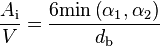
To make a distinction between the hydraulic diameter, that includes all the surfaces of the flow channel and is used to calculate the pressure drop along the length of the channel, a new parameter, called thermal diameter  [m], is defined analogously to the hydraulic diameter above. Instead of using the wetted perimeter, [m], and wetted surface area, [m2], the thermal diameter is defined using the heated perimeter,
  [m], and heated surface area,
  [m2]:
[m2]:
-
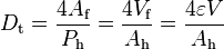
(98)
Surface heat transfer
The RPI wall boiling model is a mechanistic model developed at Rensselaer Polytechnic Institute [8], in which the wall heat flux has been divided into three separate parts: single-phase convective heat flux into liquid outside the influence of the nucleation sites (convection), convective heat flux enhanced by the detaching bubbles within the influence of the nucleation sites (quenching) and evaporation heat transfer directly into vapor through a superheated liquid microlayer (evaporation). The main idea of mechanistic boiling models is to identify the separate mechanisms that affect the heat transfer and to handle them separately, in order to better account for the various multidimensional phenomena related to two-phase flows. Such models should therefore be less dependent, for example, on flow conditions and the geometry being modeled.
The RPI boiling model was originally developed for the subcooled boiling regime inside vertical tubes. With certain modifications, such as the choice of model correlations and the addition of heat flux partitioning, it has been extended to nucleate boiling regime, and even conditions approaching dry-out.
In the original model [8] the wall heat flux,  [W/m2], is partitioned into three parts, as follows
-
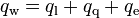
(99)
where:

convective heat flux to the liquid phase outside the zone of influence of the detaching bubbles [W/m2], 
convective heat flux to the liquid phase enhanced by detaching bubbles (quenching) [W/m2] and 
evaporation heat flux directly to the vapor phase [W/m2].
The wall surface area is divided into two fractions: an area fraction affected,  [-], and unaffected,
  [-], by the departure of the bubbles.
-
(100)
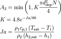
The area fraction influenced by boiling, [-], is calculated from bubble departure diameter,  [m], nucleation site density,
  [1/m2], and a correction proposed by Del Valle and Kenning [9], [-]. It is limited to less than unity.
-
(101)
The area fraction unaffected by boiling is then calculated by subtracting the affected area fraction from unity, but due to numerical reasons a lower limit of 10-4 has been set.
-

(102)
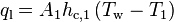
The convective heat flux to the liquid phase can then be calculated from the area fraction unaffected by boiling, [-], surface temperature,  [K], bulk liquid temperature,
  [K], and the convective heat transfer coefficient,
  [W/m2K].
-
(103)
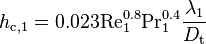
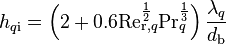
Here the convective heat transfer coefficient, [W/m2K], is calculated based on the Dittus and Boelter equation, as introduced by McAdams[10].
-
(104)
The phasic Reynolds and Prandtl numbers are defined, respectively, as follows
-
(105)
-
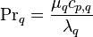
(106)
where  thermal conductivity of phase q [W/m K],
  dynamic viscosity of phase q [Ns/m2], density of phase q [kg/m3],
  specific isobaric heat capacity of phase q [J/kgK], thermal diameter [m], and velocity of phase q [m/s].
The quenching heat flux is calculated from an equation identical in form to Equation 103
-
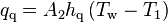
(107)
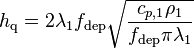
The quenching heat transfer coefficient,  , is taken according to Del Valle and Kenning [9]:
-
(108)
The evaporation heat flux is the product of evaporation mass flux and the difference between saturated vapor enthalpy and liquid enthalpy:
-
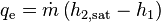
(109)
Here the evaporation mass flux,  [kg\m2s], can be written in terms of nucleation site density, [1\m2], bubble departure frequency,
  [1/s], bubble departure diameter, [m], and vapor density,
  [kg\m3].
-
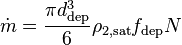
(110)
Next, the model correlations implemented for the terms appearing in the preceding equations are listed. Bubble departure frequency is calculated according to the presentation of Cole[11]:
-
(111)
Bubble departure diameter is taken according to Tolubinski and Kostanchuk [12]:
-
![d_{\text{dep}} = \text{max} \left[ \text{min} \left( d_{\text{ref}} \; e^{-\frac{T_{\text{sat}} - T_1}{{\Delta T}_{\text{ref}}}}, d_{\text{max}} \right), d_{\text{min}} \right]](/kraken/images/math/8/1/9/819603cf745bc719516648a924c6dc57.png)
(112)
where  = 45 K,
  = 0.6e-3 m,
  = 1.0e-6 m, and
  = 1.4e-3 m.
Nucleation site density, as presented by Lemmert and Chawla [13]
-
![N = \left[ 210 \left( T_{\text{w}} - T_{\text{sat}} \right) \right]^{1.805}](/kraken/images/math/2/b/a/2ba1914c4ca9b7f573ce5bbb0b5eb467.png)
(113)
is slightly modified to remove the fractional powers of temperature
-
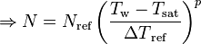
(114)
where 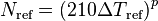 , = 10 K, and = 1.805.
Finally, an additional level of partitioning is introduced to extend applicability towards high void fractions:
-

(115)
where  is a coefficient that defines the fraction of the heat flux that is transferred to the liquid phase (liquid fraction) [-] and
  is the convective heat flux to the vapor phase [W/m2].
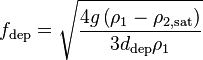
The liquid fraction, , is calculated according to the presentation of Lavieville et al. [14]:
-
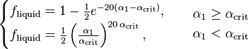
(116)
where  is the liquid volume fraction [-] and
  is the critical liquid volume fraction provided by the user. Lavieville et al. proposed a critical liquid volume fraction of
  .
.
Convective heat flux to the vapor phase is calculated similar to Equation 103
-

(117)
and the convective heat transfer coefficient,  [W/m2K], is also calculated based on the Dittus and Boelter equation [10].
-
(118)
The wall heat flux, in Equation 115, needs to be transformed into a form in which it can be casted as a source term to the relevant enthalpy equations. This is achieved by multiplying the surface heat fluxes by the ratio of heated surface area and volume,  [1/m]. There are several ways the heat flux can be distributed between the phases (and the phase interface), but the chosen one is capable of producing vapor in subcooled conditions (subcooled boiling).
-
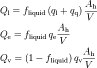
(119)
Here,  [W/m3] is added to the liquid enthalpy equations,
  [W/m3] is added to the vapor enthalpy equations, and
  [W/m3] is added to the phase interface, as shown in the following subsection. Using the definition of the thermal diameter in Equation 98, the volumetric heat fluxes in Equation 119 can be written in a more useful form:
-
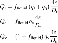
(120)
Interfacial heat transfer
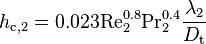
The heat transfer coefficient from phase q to the interface between the two phases,  [W/m2K], is calculated according to the correlation of Ranz and Marshall [15]:
-
(121)
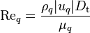
where  is the relative Reynolds number for phase q
-
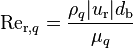
(122)
and  is the phasic Prandtl number in Equation 106,
  is the thermal conductivity of phase q [W/m K], is the density of phase q [kg/m3], dynamic viscosity of phase q [Ns/m2],
  is the bubble diameter [m], and
  is the velocity difference between the phases,
  [m/s].
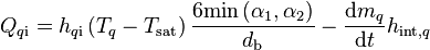
The interfacial volumetric heat fluxes from phase q to the interface between the phases,  [W/m3], are calculated from the following relation:
-
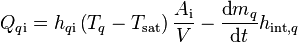
(123)
where is the interfacial heat transfer coefficient [W/m2K],  is the temperature of phase q [K],
  is the saturation temperature [K],
  is the interface area density [1/m],
  is the mass transfer rate to phase q [kg/m3s], and
  is the enthalpy of phase q at the interface [J/kg]. The last term on the right-hand side is due to phase change.
A rough approximation for the interface area density is obtained by assuming spherical bubbles and droplets with a constant diameter, [m], and assuming that the flow regime changes from bubbly flow to droplet flow at a vapor fraction of  .
.
-
(124)
When Equation 124 is combined with Equation 123, the interfacial volumetric heat fluxes are reduced to:
-
(125)
Mass transfer
By enforcing energy balance on the phase interface, i.e. setting the sum of heat fluxes to the interface equal to zero, allows for the mass transfer rate to be solved from the resulting equation.
-
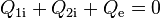
(126)
-

(127)
Denoting volumetric evaporation rate [kg/m3s], i.e. volumetric mass transfer rate from phase 1 to phase 2, as  leads to
-

(128)
-

(129)
The interfacial enthalpies are upwinded based on the direction of mass transfer:
-
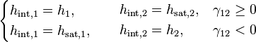
(130)
References
- ↑ Rhie, C. M., Chow, W. L., Numerical study of the turbulent flow past an airfoil with trailing edge separation. AIAA journal 21 (11), pp. 1525-1532, 1983.
- ↑ 2.0 2.1 Patankar, S. V., Numerical Heat Transfer and Fluid Flow. Hemisphere Publishing Corporation. 1980.
- ↑ Majumdar, S., Role of underrelaxation in momentum interpolation for calculation of flow with nonstaggered grids. Numerical Heat Transfer 13 (1), pp. 125-132, 1988.
- ↑ Choi, S. K., Note on the use of momentum interpolation method for unsteady flows. Numerical Heat Transfer: Part A: Applications 36 (5), pp. 545-550, 1999.
- ↑ 5.0 5.1 5.2 Pascau, A., Cell face velocity alternatives in a structured colocated grid for the unsteady navier-stokes equations. International Journal for Numerical Methods in Fluids 65 (7), pp. 812-833, 2011.
- ↑ 6.0 6.1 Kunz, R. F., Siebert, B. W., Cope, W. K., Foster, N. F., Antal, S. P., Ettorre, S. M., A coupled phasic exchange algorithm for three–dimensional multi–field analysis of heated flows with mass transfer. Computers & Fluids 27 (7), pp. 741–768, 1998.
- ↑ 7.0 7.1 Vasquez, S. A., Ivanov, V. A., A phase coupled method for solving multiphase problems in unstructured meshes. In: Proceedings of ASME FEDSM’00: ASME 2000 fluids engineering division summer meeting, Boston. pp. 743-748, 2000.
- ↑ 8.0 8.1 Kurul, N., Podowski, M. Z., On the Modeling of Multidimensional Effects in Boiling Channels. In: ANS Proceedings of 1991 National Heat Transfer Conference, Minneapolis, Minnesota, Vol. 5. pp. 30-40, 1991. ISBN: 0-89448-162-2
- ↑ 9.0 9.1 Del Valle M., V. H., Kenning, D. B. R., Subcooled flow boiling at high heat flux. Int. J. Heat Mass Transfer, Vol. 28, No. 10, pp.1907-1920, 1985.
- ↑ McAdams, W. H., Heat Transmission, 2nd Edition, McGraw-Hill, New York, 1942.
- ↑ Cole, R., A photographic study of pool boiling in the region of CHF. AIChEJ, 6 pp. 533-542, 1960.
- ↑ Tolubinski, V. I., Kostanchuk, D. M., Vapour bubbles growth rate and heat transfer intensity at subcooled water boiling, 4th. International Heat Transfer Conference, Paris, France, 1970.
- ↑ Lemmert, M., Chawla, J. M., Influence of flow velocity on surface boiling heat transfer coefficient. Heat Transfer and Boiling, Academic Press, 1977.
- ↑ Lavieville, J., Quemerais, E., Mimouni, S., Boucker, M., Mechitoua, N., NEPTUNE CFD V1.0 theory manual. NEPTUNE report Nept_2004_L1, 2(3), 2006.
- ↑ Ranz, W. E., Marshall, W. R. Jr., Evaporation from Drops, Part 2. Chemical Engineering Progress, Vol. 48, No. 4, pp. 173-180, 1952.
Cite error: <ref> tag with name "Incropera2002a" defined in <references> is not used in prior text.
Cite error: <ref> tag with name "Incropera2002b" defined in <references> is not used in prior text.