Difference between revisions of "Regular Hex Mesh coolant IFC example"
(→Files) |
(→input_sample1.m) |
||
| Line 172: | Line 172: | ||
=== input_sample1.m === | === input_sample1.m === | ||
| + | |||
| + | We used the [[Input syntax manual#sample|sample]]-card to take a sample of the material temperatures and densities on the z-axis to ensure that the interface data is read correctly by Serpent. The contents of this file are | ||
| + | |||
| + | <nowiki>SAMPLE_X = [ | ||
| + | 0.00000E+00 | ||
| + | ]; | ||
| + | |||
| + | SAMPLE_Y = [ | ||
| + | 0.00000E+00 | ||
| + | ]; | ||
| + | |||
| + | SAMPLE_Z = [ | ||
| + | -4.99000E+01 -3.88111E+01 -2.77222E+01 -1.66333E+01 -5.54444E+00 5.54444E+00 1.66333E+01 2.77222E+01 3.88111E+01 4.99000E+01 | ||
| + | ]; | ||
| + | |||
| + | sampled_T = [ | ||
| + | 5.20000E+02 5.20000E+02 5.25000E+02 5.25000E+02 5.30000E+02 5.30000E+02 5.35000E+02 5.35000E+02 5.40000E+02 5.40000E+02 | ||
| + | ]; | ||
| + | |||
| + | |||
| + | sampled_T = reshape(sampled_T, [1, 1, 10]); | ||
| + | |||
| + | sampled_rho = [ | ||
| + | -1.00000E+00 -1.00000E+00 -9.00000E-01 -9.00000E-01 -8.00000E-01 -8.00000E-01 -7.00000E-01 -7.00000E-01 -6.00000E-01 -6.00000E-01 | ||
| + | ]; | ||
| + | |||
| + | |||
| + | sampled_rho = reshape(sampled_rho, [1, 1, 10]);</nowiki> | ||
| + | |||
| + | Comparing the (Z, T, rho) triplets, we can see that the temperatures and densities are seen by Serpent as we intended. Of course, a much higher resolution could be used in sampling to ensure that the transition between the axial layers happens at the correct position. | ||
| + | |||
| + | === Geometry and mesh plots === | ||
| + | |||
| + | {|class="wikitable" style="text-align: left;" | ||
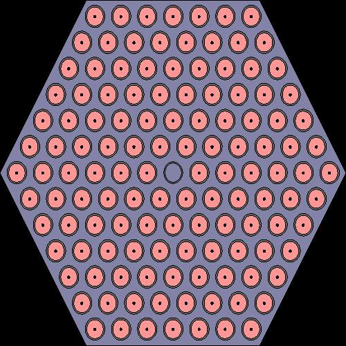
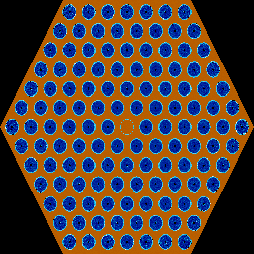
| + | |[[File:HexIFC2_geom1.png|300px|frame|left|<tt>input_geom1.png</tt>: Geometry plot in XY.]] | ||
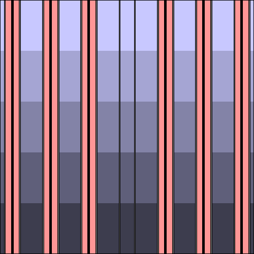
| + | |[[File:HexIFC2_geom2.png|300px|frame|left|<tt>input_geom2.png</tt>: Geometry plot in YZ.]] | ||
| + | |- | ||
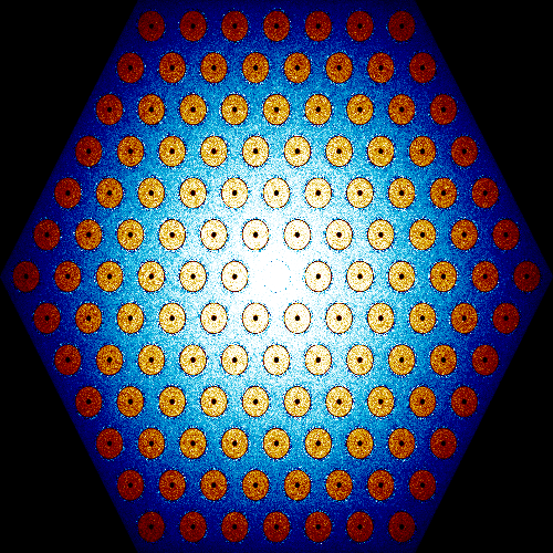
| + | |[[File:HexIFC2_mesh1.png|300px|frame|left|<tt>input_mesh1.png</tt>: Fission rate/thermal flux mesh plot in XY.]] | ||
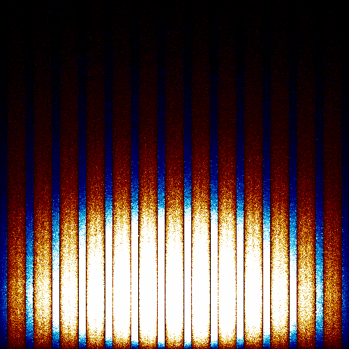
| + | |[[File:HexIFC2_mesh2.png|300px|frame|left|<tt>input_mesh2.png</tt>: Fission rate/thermal flux mesh plot in YZ.]] | ||
| + | |- | ||
| + | |[[File:HexIFC2_mesh3.png|300px|frame|left|<tt>input_mesh3.png</tt>: Interface material temperature mesh plot in XY.]] | ||
| + | |[[File:HexIFC2_mesh4.png|300px|frame|left|<tt>input_mesh4.png</tt>: Interface material temperature mesh plot in YZ.]] | ||
| + | |} | ||
Revision as of 12:33, 8 March 2018
Input example for single assembly regular mesh based interface for coolant using hexagonal mesh. On-the-fly interpolation of thermal scattering data is used for the hydrogen-1 in coolant (see therm).
Remember to add cross section libraries to the main input using set acelib.
Contents
Files
Main input
set title "Regular hex mesh interface input"

%%%%%%%%%%%%%%%%%%%%%%%%%%%%
% --- Material definitions %
%%%%%%%%%%%%%%%%%%%%%%%%%%%%

mat fuel -10.31341 rgb 255 150 150
U-234.03c 5.0131e-06
U-235.03c 5.7503e-04
U-238.03c 2.2625e-02
O-16.03c 4.5895e-02
O-17.03c 1.7482e-05

mat zirc  -6.55 rgb 100 100 100
O-16.03c 3.0743e-04
O-17.03c 1.1711e-07
%O-18.03c 6.3176e-07
Cr-50.03c 3.2962e-06
Cr-52.03c 6.3564e-05
Cr-53.03c 7.2076e-06
Cr-54.03c 1.7941e-06
Fe-54.03c 8.6699e-06
Fe-56.03c 1.3610e-04
Fe-57.03c 3.1431e-06
Fe-58.03c 4.1829e-07
Zr-90.03c 2.1827e-02
Zr-91.03c 4.7600e-03
Zr-92.03c 7.2758e-03
Zr-94.03c 7.3734e-03
Zr-96.03c 1.1879e-03
Sn-112.03c 4.6735e-06
Sn-114.03c 3.1799e-06
Sn-115.03c 1.6381e-06
Sn-116.03c 7.0055e-05
Sn-117.03c 3.7003e-05
Sn-118.03c 1.1669e-04
Sn-119.03c 4.1387e-05
Sn-120.03c 1.5697e-04
Sn-122.03c 2.2308e-05
Sn-124.03c 2.7897e-05

mat cool  sum rgb 200 200 255 moder HinWater 1001
H-1.03c 4.9457e-02
H-2.03c 7.4196e-06
O-16.03c 2.4672e-02
O-17.03c 9.3982e-06
%O-18.03c 5.0701e-05

% --- Use on-the-fly interpolation for thermal scattering data
%     lwj3.07t = 474 K / JEFF3.1.1
%     lwj3.09t = 524 K / JEFF3.1.1
%     lwj3.11t = 574 K / JEFF3.1.1

therm HinWater 0 lwj3.07t lwj3.09t lwj3.11t

%%%%%%%%%%%%%%%%%%%%%%%%%%%
% --- Geometry definition %
%%%%%%%%%%%%%%%%%%%%%%%%%%%

surf s01  hexyc 0 0 7
surf s02  pz -50
surf s03  pz  50
surf sINF inf

% --- Core

cell c01 0 fill lPIN -s01 s02 -s03
cell c02 0 outside    s01 s02 -s03
cell c03 0 outside       -s02
cell c04 0 outside             s03

% --- Fuel assembly pin lattice

lat lPIN 2 0.0 0.0 15 15 1.22
ww ww ww ww ww ww ww ww ww ww ww ww ww ww ww
 ww ww ww ww ww ww ww PF PF PF PF PF PF PF ww
  ww ww ww ww ww ww PF PF PF PF PF PF PF PF ww
   ww ww ww ww ww PF PF PF PF PF PF PF PF PF ww
    ww ww ww ww PF PF PF PF PF PF PF PF PF PF ww
     ww ww ww PF PF PF PF PF PF PF PF PF PF PF ww
      ww ww PF PF PF PF PF PF PF PF PF PF PF PF ww
       ww PF PF PF PF PF PF IT PF PF PF PF PF PF ww
        ww PF PF PF PF PF PF PF PF PF PF PF PF ww ww
         ww PF PF PF PF PF PF PF PF PF PF PF ww ww ww
          ww PF PF PF PF PF PF PF PF PF PF ww ww ww ww
           ww PF PF PF PF PF PF PF PF PF ww ww ww ww ww
            ww PF PF PF PF PF PF PF PF ww ww ww ww ww ww
             ww PF PF PF PF PF PF PF ww ww ww ww ww ww ww
              ww ww ww ww ww ww ww ww ww ww ww ww ww ww ww


% --- Pin definitions

%     Empty lattice position

pin ww
cool

%     Fuel pin

pin      PF
void     0.07
fuel     0.3765
void     0.3865
zirc     0.4575
cool

%      Instrumentation tube

pin      IT
cool     0.3850
zirc     0.4400
cool

%%%%%%%%%%%%%%%%%%%%%%%%
% --- Some run options %
%%%%%%%%%%%%%%%%%%%%%%%%

set pop 5000 1000 50

% --- Cross section libraries

%set acelib ""

% --- Geometry plot

plot 3 500 500
plot 1 500 500

% --- Sample temperature and density data in 20 points on z-axis

sample 1 0 0 1 0 0 10 -49.9 49.9

% --- Fission rate / thermal flux plot

mesh    3 500 500
mesh    1 500 500

% --- Interface temperature plot

mesh 10 3 500 500
mesh 10 1 500 500

% --- Include interface for assembly-wise fuel temperature

ifc "./coolant.ifc"
coolant.ifc
The interface consists of five axial layers from bottom to top. Here the mesh type 4 is similar to the lattice type 2 in the input (used for the lPIN lattice), although a cartesian mesh could have also been used as there is no variation in the horizontal direction. We let the coolant density decrease from 1 g/cm3 to 0.6 g/cm3 while increasing the coolant temperature from 520 K to 540 K.
2 cool 0
4
0 0 14 -50.0 50.0 1 1 5
-1.0 520
-0.9 525
-0.8 530
-0.7 535
-0.6 540
Output files
input_sample1.m
We used the sample-card to take a sample of the material temperatures and densities on the z-axis to ensure that the interface data is read correctly by Serpent. The contents of this file are
SAMPLE_X = [
 0.00000E+00
];

SAMPLE_Y = [
 0.00000E+00
];

SAMPLE_Z = [
-4.99000E+01 -3.88111E+01 -2.77222E+01 -1.66333E+01 -5.54444E+00  5.54444E+00  1.66333E+01  2.77222E+01  3.88111E+01  4.99000E+01
];

sampled_T = [
 5.20000E+02  5.20000E+02  5.25000E+02  5.25000E+02  5.30000E+02  5.30000E+02  5.35000E+02  5.35000E+02  5.40000E+02  5.40000E+02
];


sampled_T = reshape(sampled_T, [1, 1, 10]);

sampled_rho = [
-1.00000E+00 -1.00000E+00 -9.00000E-01 -9.00000E-01 -8.00000E-01 -8.00000E-01 -7.00000E-01 -7.00000E-01 -6.00000E-01 -6.00000E-01
];


sampled_rho = reshape(sampled_rho, [1, 1, 10]);
Comparing the (Z, T, rho) triplets, we can see that the temperatures and densities are seen by Serpent as we intended. Of course, a much higher resolution could be used in sampling to ensure that the transition between the axial layers happens at the correct position.
