Difference between revisions of "Input syntax manual"
(→set trc) |
|||
| Line 10: | Line 10: | ||
This page will contain the whole input syntax of Serpent 2, with links to more detailed descriptions where needed. For reference see also the Serpent 1 input manual<ref name="manual">Leppänen, J. | This page will contain the whole input syntax of Serpent 2, with links to more detailed descriptions where needed. For reference see also the Serpent 1 input manual<ref name="manual">Leppänen, J. | ||
| − | ''"Serpent – a Continuous-energy Monte Carlo Reactor Physics Burnup Calculation Code."'' [ | + | ''"Serpent – a Continuous-energy Monte Carlo Reactor Physics Burnup Calculation Code."'' [https://serpent.vtt.fi/serpent/download/Serpent_manual.pdf User manual], June 18, 2015.</ref>. |
| − | == Input cards == | + | == Input cards<span id="input cards"></span> == |
NOTE: Serpent command words are in <tt>'''boldface'''</tt> and input parameters entered by the user in <tt>''CAPITAL ITALIC''</tt>. Optional input parameters are enclosed in [ square brackets ], and when the number of values is not fixed, the remaining values are marked with three dots (...). | NOTE: Serpent command words are in <tt>'''boldface'''</tt> and input parameters entered by the user in <tt>''CAPITAL ITALIC''</tt>. Optional input parameters are enclosed in [ square brackets ], and when the number of values is not fixed, the remaining values are marked with three dots (...). | ||
| Line 18: | Line 18: | ||
=== branch (branch definition)<span id="branch"></span> === | === branch (branch definition)<span id="branch"></span> === | ||
| − | '''branch''' ''NAME'' [ '''repm''' ''MAT<sub>1</sub>'' ''MAT<sub>2</sub>'' ] | + | '''branch''' ''NAME'' [ [[#branch_repm|'''repm''']] ''MAT<sub>1</sub>'' ''MAT<sub>2</sub>'' ] |
| − | [ '''repu''' ''UNI<sub>1</sub>'' ''UNI<sub>2</sub>'' ] | + | [ [[#branch_repu|'''repu''']] ''UNI<sub>1</sub>'' ''UNI<sub>2</sub>'' ] |
| − | [ '''stp''' ''MAT DENS TEMP THERM<sub>1</sub> SABL<sub>1</sub> SABH<sub>1</sub> THERM<sub>2</sub> SABL<sub>2</sub> SABH<sub>2</sub> ...'' ] | + | [ [[#branch_stp|'''stp''']] ''MAT DENS TEMP THERM<sub>1</sub> SABL<sub>1</sub> SABH<sub>1</sub> THERM<sub>2</sub> SABL<sub>2</sub> SABH<sub>2</sub> ...'' ] |
| − | [ '''tra''' ''TGT TRANS'' ] | + | [ [[#branch_tra|'''tra''']] ''TGT TRANS'' ] |
| − | [ '''xenon''' ''OPT'' ] | + | [ [[#branch_xenon|'''xenon''']] ''OPT'' ] |
| − | [ '''samarium''' ''OPT'' ] | + | [ [[#branch_samarium|'''samarium''']] ''OPT'' ] |
| − | [ '''var''' ''VNAME VAL'' ] | + | [ [[#branch_norm|'''norm''']] ''NSF'' ] |
| − | Defines the variations invoked for a branch in the automated burnup sequence. | + | [ [[#branch_gcu|'''gcu''']] ''UNI<sub>2</sub>'' ] |
| + | [ [[#branch_reptrc|'''reptrc''']] ''FILE<sub>1</sub>'' ''FILE<sub>2</sub>'' ] | ||
| + | [ [[#branch_var|'''var''']] ''VNAME VAL'' ] | ||
| + | [ [[#branch_incl|'''incl''']] ''MODFILE'' ] | ||
| + | Defines the variations invoked for a branch in the automated burnup sequence. The first parameter: | ||
{| | {| | ||
| <tt>''NAME''</tt> | | <tt>''NAME''</tt> | ||
| : branch name | | : branch name | ||
| − | | | + | |} |
| + | |||
| + | The remaining parameters are defined by separate key words followed by the input values. | ||
| + | |||
| + | <u>Notes:</u> | ||
| + | |||
| + | *The branch card can be combined with the [[#coef (coefficient matrix definition)|coef card]], [[#hisv (history variation matrix definition)|hisv card]], and [[#casematrix (casematrix definition)| casematrix card]]. | ||
| + | *The branch name identifies the branch <tt>''BR<sub>m,i</sub>''</tt> in the variation matrix defined by the [[#coef (coefficient matrix definition)|coef card]], [[#hisv (history variation matrix definition)|hisv card]], and [[#casematrix (casematrix definition)| casematrix card]]. | ||
| + | *The input parameters consist of a number variations, which are invoked when the branch is applied. | ||
| + | *A single branch card may include one or several variations. | ||
| + | *For more information, see detailed description on the [[automated burnup sequence]]. | ||
| + | |||
| + | |||
| + | <u>Variation types:</u> | ||
| + | |||
| + | Branch material variation (<tt>'''repm'''</tt>):<span id="branch_repm"></span> | ||
| + | |||
| + | {| | ||
| <tt>''MAT<sub>1</sub>''</tt> | | <tt>''MAT<sub>1</sub>''</tt> | ||
| : name of the replaced material | | : name of the replaced material | ||
| Line 36: | Line 57: | ||
| <tt>''MAT<sub>2</sub>''</tt> | | <tt>''MAT<sub>2</sub>''</tt> | ||
| : name of the replacing material | | : name of the replacing material | ||
| − | |- | + | |} |
| + | |||
| + | <u>Notes:</u> | ||
| + | *The material variation can be used to replace one material with another, for example, to change coolant boron concentration. | ||
| + | *The material replacement works as if <tt>''MAT<sub>1</sub>''</tt> were created using the [[#mat_.28material_definition.29|mat]] or [[#mix_.28mixture_definition.29|mix]] card of <tt>''MAT<sub>2</sub>''</tt>. | ||
| + | *The name of the material present in the geometry will still be <tt>''MAT<sub>1</sub>''</tt> after the replacement, but the material specification (composition, density, tmp, moder, rgb, etc.) will correspond to <tt>''MAT<sub>2</sub>''</tt>. | ||
| + | **This means that all other input-cards that are linked to a specific material name such as '''dm''' entry in the [[#det_dm|det card]], '''sm''' entry in the [[#src_sm|src card]], [[#set_trc|set trc]] option and/or [[#set_iter_nuc|set iter nuc]] option can be linked to the original material (<tt>''MAT<sub>1</sub>''</tt>) and they will automatically apply to whatever material <tt>''MAT<sub>2</sub>''</tt> replaces <tt>''MAT<sub>1</sub>''</tt> for the branch calculation. | ||
| + | *The replaced material ''MAT<sub>1</sub>'' is also replaced inside mixtures. | ||
| + | **This means one can not replace a material with a mixture defined with [[#mix (mixture_definition)|mix card]] containing the replaced material (for example replacing pure water defined with [[#mat (material definition)|mat card]] by a mixture of boron and water defined with a [[#mix (mixture definition)|mix card]] containing the same pure water material). | ||
| + | *The replacing material ''MAT<sub>2</sub>'' can not be included in the geometry using other cards than the branch card, from version 2.1.30 and on. | ||
| + | |||
| + | |||
| + | Branch universe variation (<tt>'''repu'''</tt>):<span id="branch_repu"></span> | ||
| + | |||
| + | {| | ||
| <tt>''UNI<sub>1</sub>''</tt> | | <tt>''UNI<sub>1</sub>''</tt> | ||
| : name of the replaced universe | | : name of the replaced universe | ||
| Line 42: | Line 77: | ||
| <tt>''UNI<sub>2</sub>''</tt> | | <tt>''UNI<sub>2</sub>''</tt> | ||
| : name of the replacing universe | | : name of the replacing universe | ||
| − | |- | + | |} |
| + | |||
| + | <u>Notes:</u> | ||
| + | *The universe variation can be used to replace one universe with another, for example, to replace empty control rod guide tubes with rodded tubes for control rod insertion in 2D geometries. | ||
| + | *The name of the universe present in the geometry will still be <tt>''UNI<sub>1</sub>''</tt> after the replacement, but the universe contents will correspond to <tt>''UNI<sub>2</sub>''</tt>. | ||
| + | *This means that all other input-cards that are linked to a specific universe name such as '''du''' entry in the [[#det_du|det card]] and/or '''su''' entry in the [[#src_su|src card]] can be linked to the original universe (<tt>''UNI<sub>1</sub>''</tt>) and they will automatically apply to whatever universe <tt>''UNI<sub>2</sub>''</tt> replaces <tt>''UNI<sub>1</sub>''</tt> for the branch calculation. | ||
| + | |||
| + | |||
| + | Branch state variation, density/temperature (<tt>'''stp'''</tt>):<span id="branch_stp"></span> | ||
| + | {| | ||
| <tt>''MAT''</tt> | | <tt>''MAT''</tt> | ||
| : name of the material for which density and temperature are adjusted | | : name of the material for which density and temperature are adjusted | ||
|- | |- | ||
| <tt>''DENS''</tt> | | <tt>''DENS''</tt> | ||
| − | | : material density after adjustment (positive | + | | : material density after adjustment (positive value = atomic density [in b<sup>-1</sup>cm<sup>-1</sup>], negative value = mass density [in g/cm<sup>3</sup>]) |
|- | |- | ||
| <tt>''TEMP''</tt> | | <tt>''TEMP''</tt> | ||
| − | | : material temperature after adjustment | + | | : material temperature after adjustment [in K] |
|- | |- | ||
| <tt>''THERM<sub>n</sub>''</tt> | | <tt>''THERM<sub>n</sub>''</tt> | ||
| − | | : ''n | + | | : ''n''-th thermal scattering data associated with the material |
|- | |- | ||
| <tt>''SABL<sub>n</sub>''</tt> | | <tt>''SABL<sub>n</sub>''</tt> | ||
| − | | : name of the ''n'' | + | | : name of the ''n''-th S(α, β) library for temperature below the given value |
|- | |- | ||
| <tt>''SABH<sub>n</sub>''</tt> | | <tt>''SABH<sub>n</sub>''</tt> | ||
| − | | : name of the ''n'' | + | | : name of the ''n''-th S(α, β) library for temperature above the given value |
| − | |- | + | |} |
| + | |||
| + | <u>Notes:</u> | ||
| + | *The state variation can be used to change material density and temperature. | ||
| + | *There is a special entry for the <tt>''TEMP''</tt> parameter: | ||
| + | **"<tt>-1</tt>": to not adjust temperature | ||
| + | *There are two special entries for the <tt>''DENS''</tt> parameter: | ||
| + | ** "<tt>sum</tt>": to define the material density as the sum of the constituent nuclides densities (not supported from version 2.2.0 and on) | ||
| + | ** "<tt>original</tt>": to keep unmodified the material density (introduced in version 2.2.1). | ||
| + | *The adjustment is made using the built-in [[Doppler-broadening preprocessor routine]] and tabular interpolation for S(α, β) thermal scattering data. | ||
| + | *The last three parameters of the card are provided only if the material has thermal scattering libraries attached to it (see the [[#therm (thermal scattering library definition)|therm card]]). | ||
| + | |||
| + | |||
| + | Branch transformation variation (<tt>'''tra'''</tt>):<span id="branch_tra"></span> | ||
| + | |||
| + | {| | ||
| <tt>''TGT''</tt> | | <tt>''TGT''</tt> | ||
| : target universe, surface or cell | | : target universe, surface or cell | ||
| Line 66: | Line 125: | ||
| <tt>''TRANS''</tt> | | <tt>''TRANS''</tt> | ||
| : name of the applied transformation | | : name of the applied transformation | ||
| − | | | + | |} |
| + | |||
| + | <u>Notes:</u> | ||
| + | *The transformation variation can be used to move or rotate different parts of the geometry, for example, to adjust the position of control rods in 3D geometries. | ||
| + | *The name of the transformation <tt>''TRANS''</tt> refers to the unit (universe, cell or surface) entry in the [[#trans (transformations)|trans card]]. | ||
| + | |||
| + | |||
| + | Branch xenon variation (<tt>'''xenon'''</tt>):<span id="branch_xenon"></span> | ||
| + | |||
| + | {| | ||
| <tt>''OPT''</tt> | | <tt>''OPT''</tt> | ||
| − | | : option for setting poison concentrations (0 = set to zero, 1 = use values from restart file) | + | | : option for setting xenon poison concentrations (0 = set to zero, 1 = use values from restart file) |
| + | |} | ||
| + | |||
| + | <u>Notes:</u> | ||
| + | *The xenon variation can be set to enforced the Xe-135 and Xe-135m concentrations and optionally I-135 concentration to zero. | ||
| + | **By default the concentrations are read from the restart file. | ||
| + | *Equilibrium xenon ([[#set_xenon|set xenon]] option). | ||
| + | **If the calculation is "<tt>on</tt>", then the option "<tt>0</tt>" sets I-135, Xe-135 and Xe-135m concentrations to zero. | ||
| + | **If the calculation is "<tt>off</tt>", then the option "<tt>0</tt>" sets only Xe-135 and Xe-135m concentrations to zero. | ||
| + | |||
| + | |||
| + | Branch samarium variation (<tt>'''samarium'''</tt>):<span id="branch_samarium"></span> | ||
| + | |||
| + | {| | ||
| + | | <tt>''OPT''</tt> | ||
| + | | : option for setting samarium poison concentrations (0 = set to zero, 1 = use values from restart file) | ||
| + | |} | ||
| + | |||
| + | <u>Notes:</u> | ||
| + | *The samarium variation can be set to enforce the Sm-149 concentration and possibly Pm-149 concentration to zero. | ||
| + | **By default the concentrations are read from the restart file. | ||
| + | *Equilibrium samarium ([[#set_samarium|set samarium]] option): | ||
| + | **If the calculation is "<tt>on</tt>", then the option "<tt>0</tt>" sets both Pm-149 and Sm-149 concentrations to zero. | ||
| + | **If the calculation is "<tt>off</tt>", then the option "<tt>0</tt>" sets only Sm-149 concentration to zero. | ||
| + | |||
| + | |||
| + | Branch normalization variation (<tt>'''nsf'''</tt>):<span id="branch_nsf"></span> | ||
| + | |||
| + | {| | ||
| + | | <tt>''NSF''</tt> | ||
| + | | : normalization scaling factor | ||
| + | |} | ||
| + | |||
| + | <u>Notes:</u> | ||
| + | *The normalization variation can be used to change the normalization. | ||
| + | *The adjustment is made applying the parameter ''NSF'' as a multiplicative scaling factor to the given normalization. | ||
| + | |||
| + | |||
| + | Branch group constant variation (<tt>'''gcu'''</tt>):<span id="branch_gcu"></span> | ||
| + | |||
| + | {| | ||
| + | | <tt>''UNI<sub>2</sub>''</tt> | ||
| + | |: name of the replacing universe | ||
| + | |} | ||
| + | |||
| + | <u>Notes:</u> | ||
| + | *The group constant variation can be used to replace the universe for group constant generation. | ||
| + | *The variation is limited to a single-valued GCU-list (see [[#set gcu|set gcu]] option). | ||
| + | |||
| + | |||
| + | Branch transport-correction variation (<tt>'''reptrc'''</tt>):<span id="branch_reptrc"></span> | ||
| + | |||
| + | {| | ||
| + | | <tt>''FILE<sub>1</sub>''</tt> | ||
| + | | : file path of the replaced transport correction curve data | ||
|- | |- | ||
| + | | <tt>''FILE<sub>2</sub>''</tt> | ||
| + | | : file path of the replacing transport correction curve data | ||
| + | |} | ||
| + | |||
| + | <u>Notes:</u> | ||
| + | *The transport-correction variation can be used to replace a transport correction file with another (see [[#set trc|set trc]] option). | ||
| + | |||
| + | |||
| + | Branch variable variation (<tt>'''var'''</tt>):<span id="branch_var"></span> | ||
| + | |||
| + | {| | ||
| <tt>''VNAME''</tt> | | <tt>''VNAME''</tt> | ||
| : variable name | | : variable name | ||
| Line 78: | Line 211: | ||
<u>Notes:</u> | <u>Notes:</u> | ||
| + | *The variable variation can be used to pass information into the output file, which may be convenient for the post-processing of the data. | ||
| − | |||
| − | |||
| − | |||
| − | |||
| − | |||
| − | |||
| − | |||
| − | |||
| − | |||
| − | |||
| − | |||
| − | |||
| − | |||
| − | + | Branch user-defined variation (<tt>'''incl'''</tt>):<span id="branch_incl"></span> | |
| + | {| | ||
| + | | <tt>''MODFILE''</tt> | ||
| + | |: file path to an additional/modified input file | ||
| + | |} | ||
| − | + | <u>Notes:</u> | |
| + | *The user-defined variation can be used as a multi-purpose option to modify the base-input via the additional input file <tt>''MODFILE''</tt>. | ||
| − | Defines | + | === casematrix (casematrix definition)<span id="casematrix"></span> === |
| + | |||
| + | '''casematrix''' ''CASE_NAME'' | ||
| + | ''NHIS'' [ ''HIS_BR<sub>1</sub>'' ''HIS_BR<sub>2</sub>'' ... ''HIS_BR<sub>NHIS</sub>'' ] | ||
| + | ''NBU'' [ ''BU<sub>1</sub>'' ''BU<sub>2</sub>'' ... ''BU<sub>NBU</sub>'' ] | ||
| + | ''NBR<sub>1</sub>'' [ ''BR<sub>1,1</sub>'' ''BR<sub>1,2</sub>'' ... ''BR<sub>1,NBR<sub>1</sub></sub>'' ] | ||
| + | ''NBR<sub>2</sub>'' [ ''BR<sub>2,1</sub>'' ''BR<sub>2,2</sub>'' ... ''BR<sub>1,NBR<sub>2</sub></sub>'' ] | ||
| + | ... | ||
| + | |||
| + | Defines the casematrix for the automated burnup sequence. Input values: | ||
{| | {| | ||
| − | | <tt>'' | + | | <tt>''CASE_NAME''</tt> |
| − | | : | + | | : name of the casematrix |
|- | |- | ||
| − | | <tt>'' | + | | <tt>''NHIS''</tt> |
| − | | : | + | | : number of history variations |
|- | |- | ||
| − | | <tt>'' | + | | <tt>''HIS_BR<sub>k</sub>''</tt> |
| − | | : | + | | : name of the ''k''-th history variation branch |
|- | |- | ||
| − | | <tt>'' | + | | <tt>''NBU''</tt> |
| − | + | | : number of burnup points | |
| − | + | ||
| − | + | ||
| − | + | ||
| − | + | ||
| − | + | ||
| − | + | ||
| − | + | ||
| − | + | ||
| − | | : | + | |
|- | |- | ||
| − | | <tt>'' | + | | <tt>''BU<sub>n</sub>''</tt> |
| − | | : | + | | : burnup steps at which the momentary variation branches are invoked (positive value = burnup [in MWd/kg], negative value = time [in d]) |
|- | |- | ||
| − | | <tt>'' | + | | <tt>''NBR<sub>m</sub>''</tt> |
| − | | : | + | | : number branches in the ''m''-th dimension of the burnup matrix |
|- | |- | ||
| − | | <tt>'' | + | | <tt>''BR<sub>m,i</sub>''</tt> |
| − | | : | + | | : name of the ''i''-th branch in the ''m''-th dimension |
|} | |} | ||
| − | + | <u>Notes:</u> | |
| + | *The casematrix card performs multiple depletions with <tt>''NHIS''</tt> (different) historical variations and performs restarts similar as the [[#coef|coef]] input card. | ||
| + | *The casematrix card creates a multi-dimensional coefficient matrix (of size <tt>''NBR<sub>1</sub>''</tt> × <tt>''NBR<sub>2</sub>''</tt> × <tt>''NBR<sub>3</sub>''</tt> × ... ). | ||
| + | **The automated burnup sequence performs a restart for each of the listed burnup points, and loops over the branch combinations defined by the coefficient matrix. | ||
| + | **This is repeated for each different depletion history. | ||
| + | *The casematrix card is used together with the [[#branch (branch definition)|branch card]] and [[Installing_and_running_Serpent#Running_casematrix_calculations|<tt>''-casematrix''</tt>]] command line option. | ||
| + | *Multiple casematrix cards can be given in a single input file. | ||
| + | *For more information, see detailed description on [[automated burnup sequence]]. | ||
| + | |||
| + | === cell (cell definition)<span id="cell"></span> === | ||
| + | |||
| + | |||
| + | '''cell''' ''NAME UNI<sub>0</sub> MAT'' [ ''SURF<sub>1</sub>'' ''SURF<sub>2</sub>'' ... ] | ||
| − | Defines | + | Defines a cell. Input values: |
{| | {| | ||
| Line 142: | Line 280: | ||
| <tt>''UNI<sub>0</sub>''</tt> | | <tt>''UNI<sub>0</sub>''</tt> | ||
| : universe where the cell belongs to | | : universe where the cell belongs to | ||
| + | |- | ||
| + | | <tt>''MAT''</tt> | ||
| + | | : material that fills the cell | ||
|- | |- | ||
| <tt>''SURF<sub>n</sub>''</tt> | | <tt>''SURF<sub>n</sub>''</tt> | ||
| Line 148: | Line 289: | ||
<u>Notes:</u> | <u>Notes:</u> | ||
| − | + | *The cell definition is based on the universe-based geometry type in Serpent. | |
| − | * | + | *Universes are implicitly declared, e.g., by using the <tt>''UNI<sub>0</sub>''</tt> key word on cell cards, as there is no explicit universe input card. |
| − | + | *The surface list defines the boundaries of the cell by listing the surface names (as provided in the surface definition, [[#surf (surface definition)|surf card]]), together with the operator identifiers (nothing for intersection, ":" for union, "-" for complement and "#" for cell complement). | |
| + | *The general cell definition (so-called "material cell") have tailored types, defined by special material entries (replacing <tt>''MAT''</tt>): | ||
| + | ::{| class="wikitable" style="text-align: left;" | ||
| + | ! Type | ||
| + | ! Description | ||
| + | |- | ||
| + | | <tt>void</tt> | ||
| + | | region is defined as zero-collision | ||
| + | |- | ||
| + | | <tt>fill ''UNI<sub>1</sub>''</tt> | ||
| + | | region is filled by another universe, <tt>''UNI<sub>1</sub>''</tt> | ||
| + | |- | ||
| + | | <tt>outside</tt> | ||
| + | | region is not part of the actual geometry ("outside world") | ||
| + | |- | ||
| + | |} | ||
| + | ::Outside cells: | ||
| + | ::*When the particle enters an outside cell, the boundary conditions are applied (see [[#set bc|set bc]] option). It is important that the geometry model is non-re-entrant (convex) when vacuum boundary conditions are used. Delta-tracking might miss the boundary conditions in a re-entrant (concave) outer surface. | ||
| + | ::*Outside cells are allowed only in the root universe. It is important that all space outside the model is defined. | ||
| + | *Cells defined without surfaces are treated as infinite, from version 2.1.32 on. | ||
*When the geometry is set up, the root universe must always be defined. By default the root universe is named "0", and it can be changed with the [[#set root|set root]] option. | *When the geometry is set up, the root universe must always be defined. By default the root universe is named "0", and it can be changed with the [[#set root|set root]] option. | ||
| − | |||
| − | |||
| − | |||
| − | |||
*For more information, see detailed description on the [[universe-based geometry type in Serpent]]. | *For more information, see detailed description on the [[universe-based geometry type in Serpent]]. | ||
| Line 171: | Line 327: | ||
|- | |- | ||
| <tt>''BU<sub>n</sub>''</tt> | | <tt>''BU<sub>n</sub>''</tt> | ||
| − | | : burnup steps at which the branches are invoked | + | | : burnup steps at which the branches are invoked (positive value = burnup [in MWd/kg], negative value = time [in d]) |
|- | |- | ||
| <tt>''NBR<sub>m</sub>''</tt> | | <tt>''NBR<sub>m</sub>''</tt> | ||
| − | | : number branches in the ''m'' | + | | : number branches in the ''m''-th dimension of the burnup matrix |
|- | |- | ||
| <tt>''BR<sub>m,i</sub>''</tt> | | <tt>''BR<sub>m,i</sub>''</tt> | ||
| − | | : name of the ''i'' | + | | : name of the ''i''-th branch in the ''m''-th dimension |
|} | |} | ||
<u>Notes:</u> | <u>Notes:</u> | ||
| − | *The coef card creates a multi-dimensional coefficient matrix (of size <tt>''NBR<sub>1</sub>''</tt> | + | *The coef card creates a multi-dimensional coefficient matrix (of size <tt>''NBR<sub>1</sub>''</tt> × <tt>''NBR<sub>2</sub>''</tt> × <tt>''NBR<sub>3</sub>''</tt> × ... ). |
| − | + | **The automated burnup sequence performs a restart for each of the listed burnup points, and loops over the branch combinations defined by the coefficient matrix. | |
| − | *The coef card is used together with the [[#branch (branch definition)|branch card]] | + | *The coef card is used together with the [[#branch (branch definition)|branch]] card. |
| + | *For multiple historical variations or historical conditions defined using a [[#branch (branch definition)|branch]] card, see the [[#casematrix (casematrix definition)|casematrix]] card. | ||
*For more information, see detailed description on [[automated burnup sequence]]. | *For more information, see detailed description on [[automated burnup sequence]]. | ||
| + | |||
| + | === datamesh (general data mesh definition)<span id="datamesh"></span> === | ||
| + | |||
| + | '''datamesh''' ''NAME'' ''TYPE'' ''USE<sub>LC</sub>'' [ ... ] | ||
| + | |||
| + | Defines a general data mesh to be used for spacial discretisation. Input values: | ||
| + | |||
| + | {| | ||
| + | | <tt>''NAME''</tt> | ||
| + | | : mesh name | ||
| + | |- | ||
| + | | <tt>''TYPE''</tt> | ||
| + | | : mesh type | ||
| + | |- | ||
| + | | <tt>''USE<sub>LC</sub>''</tt> | ||
| + | | : use lowest level coordinates (1/yes) instead of global coordinates (0/no) for the mesh search | ||
| + | |- | ||
| + | |} | ||
| + | |||
| + | The remaining parameters are type-dependent. | ||
| + | |||
| + | <u>Notes:</u> | ||
| + | *The general data mesh can be used, e.g., with detectors ('''dmesh''' entry in the [[#det|det card]]), interfaces ([[#ifc|ifc card]]), sensitivities ('''opt dmesh''' entry in the [[#sens|sens card]]), etc. | ||
| + | *When Serpent makes the mesh search for a specific collision point, it will save the collision mesh cell temporarily so that the cell search is conducted at most once even when scoring multiple estimators using the same mesh. | ||
| + | *The nested data meshes (type 9) take the coordinates' level from the <tt>''USE<sub>LC</sub>''</tt> parameter defined in the nested mesh itself and use it in the subsequent sub-meshes, overriding the <tt>''USE<sub>LC</sub>''</tt> parameter defined on those. | ||
| + | |||
| + | The available <u>general data mesh types</u> are: | ||
| + | ::{| class="wikitable" style="text-align: left;" | ||
| + | ! Type | ||
| + | ! Description | ||
| + | |- | ||
| + | | [[#datamesh_1|<tt>1</tt>]] | ||
| + | | regular 3D Cartesian mesh | ||
| + | |- | ||
| + | | [[#datamesh_2|<tt>2</tt>]] | ||
| + | | regular 2D cylindrical mesh | ||
| + | |- | ||
| + | | [[#datamesh_4|<tt>4</tt>]] | ||
| + | | regular 3D X-type hexagonal mesh | ||
| + | |- | ||
| + | | [[#datamesh_5|<tt>5</tt>]] | ||
| + | | regular 3D Y-type hexagonal mesh | ||
| + | |- | ||
| + | | [[#datamesh_6|<tt>6</tt>]] | ||
| + | | irregular 3D Cartesian mesh | ||
| + | |- | ||
| + | | [[#datamesh_8|<tt>8</tt>]] | ||
| + | | radially irregular 2D cylindrical mesh | ||
| + | |- | ||
| + | | [[#datamesh_9|<tt>9</tt>]] | ||
| + | | regular nested mesh | ||
| + | |- | ||
| + | |} | ||
| + | |||
| + | The syntax of the available types is as follows: | ||
| + | |||
| + | '''datamesh''' ''NAME'' '''1''' ''USE<sub>LC</sub>'' ''N<sub>X</sub>'' ''X<sub>MIN</sub>'' ''X<sub>MAX</sub>'' ''N<sub>Y</sub>'' ''Y<sub>MIN</sub>'' ''Y<sub>MAX</sub>'' ''N<sub>Z</sub>'' ''Z<sub>MIN</sub>'' ''Z<sub>MAX</sub>'' <span id="datamesh_1"></span> | ||
| + | |||
| + | {| | ||
| + | | <tt>''N<sub>X</sub>''</tt> | ||
| + | | : number of cells in the x-direction | ||
| + | |- | ||
| + | | <tt>''X<sub>MIN</sub>''</tt> | ||
| + | | : mesh lower x-boundary [in cm] | ||
| + | |- | ||
| + | | <tt>''X<sub>MAX</sub>''</tt> | ||
| + | | : mesh higher x-boundary [in cm] | ||
| + | |- | ||
| + | | <tt>''N<sub>Y</sub>''</tt> | ||
| + | | : number of cells in the y-direction | ||
| + | |- | ||
| + | | <tt>''Y<sub>MIN</sub>''</tt> | ||
| + | | : mesh lower y-boundary [in cm] | ||
| + | |- | ||
| + | | <tt>''Y<sub>MAX</sub>''</tt> | ||
| + | | : mesh higher y-boundary [in cm] | ||
| + | |- | ||
| + | | <tt>''N<sub>Z</sub>''</tt> | ||
| + | | : number of cells in the z-direction | ||
| + | |- | ||
| + | | <tt>''Z<sub>MIN</sub>''</tt> | ||
| + | | : mesh lower z-boundary [in cm] | ||
| + | |- | ||
| + | | <tt>''Z<sub>MAX</sub>''</tt> | ||
| + | | : mesh higher z-boundary [in cm] | ||
| + | |} | ||
| + | |||
| + | '''datamesh''' ''NAME'' '''2''' ''USE<sub>LC</sub>'' ''N<sub>R</sub>'' ''R<sub>MIN</sub>'' ''R<sub>MAX</sub>'' ''N<sub>PHI</sub>'' <span id="datamesh_2"></span> | ||
| + | |||
| + | {| | ||
| + | | <tt>''N<sub>R</sub>''</tt> | ||
| + | | : number of cells in the radial direction | ||
| + | |- | ||
| + | | <tt>''R<sub>MIN</sub>''</tt> | ||
| + | | : mesh inner radial boundary [in cm] | ||
| + | |- | ||
| + | | <tt>''R<sub>MAX</sub>''</tt> | ||
| + | | : mesh outer radial boundary [in cm] | ||
| + | |- | ||
| + | | <tt>''N<sub>PHI</sub>''</tt> | ||
| + | | : number of cells in the polar angle direction | ||
| + | |} | ||
| + | |||
| + | [[File:Hex lattice x index.png|frame|X-type hexagonal mesh horizontal indexing example for N<sub>X</sub> = N<sub>Y</sub> = 3.]] | ||
| + | |||
| + | '''datamesh''' ''NAME'' '''4''' ''USE<sub>LC</sub>'' ''X<sub>0</sub>'' ''Y<sub>0</sub>'' ''PITCH'' ''Z<sub>MIN</sub>'' ''Z<sub>MAX</sub>'' ''N<sub>X</sub>'' ''N<sub>Y</sub>'' ''N<sub>Z</sub>'' <span id="datamesh_4"></span> | ||
| + | |||
| + | {| | ||
| + | | <tt>''X<sub>0</sub>''</tt> | ||
| + | | : mesh horizontal origin x-coordinate [in cm] | ||
| + | |- | ||
| + | | <tt>''Y<sub>0</sub>''</tt> | ||
| + | | : mesh horizontal origin y-coordinate [in cm] | ||
| + | |- | ||
| + | | <tt>''PITCH''</tt> | ||
| + | | : mesh horizontal pitch (equal to cell flat-to-flat width) [in cm] | ||
| + | |- | ||
| + | | <tt>''Z<sub>MIN</sub>''</tt> | ||
| + | | : mesh lower z-boundary [in cm] | ||
| + | |- | ||
| + | | <tt>''Z<sub>MAX</sub>''</tt> | ||
| + | | : mesh higher z-boundary [in cm] | ||
| + | |- | ||
| + | | <tt>''N<sub>X</sub>''</tt> | ||
| + | | : number of cells in the x-direction | ||
| + | |- | ||
| + | | <tt>''N<sub>Y</sub>''</tt> | ||
| + | | : number of cells in the y-direction | ||
| + | |- | ||
| + | | <tt>''N<sub>Z</sub>''</tt> | ||
| + | | : number of cells in the z-direction | ||
| + | |} | ||
| + | |||
| + | [[File:Hex lattice y index.png|frame|Y-type hexagonal mesh horizontal indexing example for N<sub>X</sub> = N<sub>Y</sub> = 3.]] | ||
| + | |||
| + | '''datamesh''' ''NAME'' '''5''' ''USE<sub>LC</sub>'' ''X<sub>0</sub>'' ''Y<sub>0</sub>'' ''PITCH'' ''Z<sub>MIN</sub>'' ''Z<sub>MAX</sub>'' ''N<sub>X</sub>'' ''N<sub>Y</sub>'' ''N<sub>Z</sub>'' <span id="datamesh_5"></span> | ||
| + | |||
| + | {| | ||
| + | | <tt>''X<sub>0</sub>''</tt> | ||
| + | | : mesh horizontal origin x-coordinate [in cm] | ||
| + | |- | ||
| + | | <tt>''Y<sub>0</sub>''</tt> | ||
| + | | : mesh horizontal origin y-coordinate [in cm] | ||
| + | |- | ||
| + | | <tt>''PITCH''</tt> | ||
| + | | : mesh horizontal pitch (equal to cell flat-to-flat width) [in cm] | ||
| + | |- | ||
| + | | <tt>''Z<sub>MIN</sub>''</tt> | ||
| + | | : mesh lower z-boundary [in cm] | ||
| + | |- | ||
| + | | <tt>''Z<sub>MAX</sub>''</tt> | ||
| + | | : mesh higher z-boundary [in cm] | ||
| + | |- | ||
| + | | <tt>''N<sub>X</sub>''</tt> | ||
| + | | : number of cells in the x-direction | ||
| + | |- | ||
| + | | <tt>''N<sub>Y</sub>''</tt> | ||
| + | | : number of cells in the y-direction | ||
| + | |- | ||
| + | | <tt>''N<sub>Z</sub>''</tt> | ||
| + | | : number of cells in the z-direction | ||
| + | |} | ||
| + | |||
| + | '''datamesh''' ''NAME'' '''6''' ''USE<sub>LC</sub>'' ''N<sub>X</sub>'' ''N<sub>Y</sub>'' ''N<sub>Z</sub>'' ''X<sub>1</sub>'' ... ''X<sub>N<sub>X</sub>+1</sub>'' ''Y<sub>1</sub>'' ... ''Y<sub>N<sub>Y</sub>+1</sub>'' ''Z<sub>1</sub>'' ... ''Z<sub>N<sub>Z</sub>+1</sub>'' <span id="datamesh_6"></span> | ||
| + | |||
| + | {| | ||
| + | | <tt>''N<sub>X</sub>''</tt> | ||
| + | | : number of cells in the x-direction | ||
| + | |- | ||
| + | | <tt>''N<sub>Y</sub>''</tt> | ||
| + | | : number of cells in the y-direction | ||
| + | |- | ||
| + | | <tt>''N<sub>Z</sub>''</tt> | ||
| + | | : number of cells in the z-direction | ||
| + | |- | ||
| + | | <tt>''X<sub>i</sub>''</tt> | ||
| + | | : <tt>''N<sub>X</sub>'' + 1</tt> mesh boundaries in the x-direction [in cm] | ||
| + | |- | ||
| + | | <tt>''Y<sub>i</sub>''</tt> | ||
| + | | : <tt>''N<sub>Y</sub>'' + 1</tt> mesh boundaries in the y-direction [in cm] | ||
| + | |- | ||
| + | | <tt>''Z<sub>i</sub>''</tt> | ||
| + | | : <tt>''N<sub>Z</sub>'' + 1</tt> mesh boundaries in the z-direction [in cm] | ||
| + | |} | ||
| + | |||
| + | '''datamesh''' ''NAME'' '''8''' ''USE<sub>LC</sub>'' ''N<sub>R</sub>'' ''N<sub>PHI</sub>'' ''R<sub>1</sub>'' ... ''R<sub>N<sub>R</sub>+1</sub>'' <span id="datamesh_8"></span> | ||
| + | |||
| + | {| | ||
| + | | <tt>''N<sub>R</sub>''</tt> | ||
| + | | : number of cells in the radial direction | ||
| + | |- | ||
| + | | <tt>''N<sub>PHI</sub>''</tt> | ||
| + | | : number of cells in the polar angle direction | ||
| + | |- | ||
| + | | <tt>''R<sub>i</sub>''</tt> | ||
| + | | : <tt>''N<sub>R</sub>'' + 1</tt> mesh boundaries in the radial direction [in cm] | ||
| + | |} | ||
| + | |||
| + | '''datamesh''' ''NAME'' '''9''' ''USE<sub>LC</sub>'' ''N<sub>LEVEL</sub>'' ''MESH<sub>1</sub>'' ... ''MESH<sub>N<sub>LEVEL</sub></sub>'' <span id="datamesh_9"></span> | ||
| + | |||
| + | {| | ||
| + | | <tt>''N<sub>LEVEL</sub>''</tt> | ||
| + | | : number of nested levels in this mesh | ||
| + | |- | ||
| + | | <tt>''MESH<sub>i</sub>''</tt> | ||
| + | | : sub mesh to use at level ''i'' | ||
| + | |} | ||
=== dep (depletion history)<span id="dep"></span> === | === dep (depletion history)<span id="dep"></span> === | ||
| Line 202: | Line 566: | ||
The possible step types are: | The possible step types are: | ||
| − | {| class="wikitable" style="text-align: left;" | + | ::{| class="wikitable" style="text-align: left;" |
! Type | ! Type | ||
! Description | ! Description | ||
| Line 250: | Line 614: | ||
<u>Notes:</u> | <u>Notes:</u> | ||
| − | * | + | *Multiple depletion histories with different step types can be specified in the input, and they will be executed in the input order. |
| − | *Transport cycle is run only once with | + | *Depletion calculations (burnup/activation steps) require normalization. |
| + | **See: [[#set power|set power]], [[#set powdens|set powdens]], [[#set flux|set flux]], [[#set genrate|set genrate]], [[#set fissrate|set fissrate]], [[#set absrate|set absrate]], [[#set lossrate|set lossrate]], [[#set srcrate|set srcrate]], [[#set sfrate|set sfrate]]. | ||
| + | **If multiple depletion histories and normalizations are defined in the input, the first normalization will be used with the first depletion history, the second normalization with the second depletion history and so on. | ||
| + | ***Note that even though decay calculations (decay steps) disregard the user defined normalization, a normalization has to be defined also for the decay history, if multiple normalizations are defined in the input and there are depletion histories (burnup/activation steps) after the decay calculation. | ||
| + | **If the normalization is set to zero, physical estimates, e.g., detectors will be printed as zero. | ||
| + | ***Alternatively, use a very small value to enforce a non-zero normalization. | ||
| + | **Except: | ||
| + | ***Radioactive decay source: source rate normalization is carried out automatically based on the total emission rate. | ||
| + | ***Decay steps: equivalent, e.g., zero power. | ||
| + | *Activation step, "<tt>actstep</tt>" and "<tt>acttot</tt>": | ||
| + | **Transport cycle is run only once and transmutation cross sections are not updated. | ||
| + | **Limitations: | ||
| + | ***It must be preceeded by a burnup step. | ||
| + | ***It cannot be used with a burnable material radioactive source. | ||
| + | ***Burnup is not calculated correctly | ||
| + | *Decay step, "<tt>decstep</tt>" and "<tt>dectot</tt>": | ||
| + | **Transport cycle is omitted and transmutation cross sections are not calculated. | ||
| + | **Limitations: | ||
| + | ***It cannot preceed activation steps. | ||
| + | ***Physical estimates, e.g., detectors will not be printed for the given step (value zero) due to normalization | ||
| − | '''dep''' '''pro''' '' | + | '''dep''' '''pro''' ''REP_NAME'' ''STYPE'' [ ''STEP<sub>1</sub> STEP<sub>2</sub> ...'' ] |
| + | |||
| + | Links a reprocessor to the depletion calculation. Input values: | ||
| + | |||
| + | {| | ||
| + | | <tt>''REP_NAME''</tt> | ||
| + | | : reprocessor name | ||
| + | |- | ||
| + | | <tt>''STYPE''</tt> | ||
| + | | : step type | ||
| + | |- | ||
| + | | <tt>''STEP<sub>n</sub>''</tt> | ||
| + | | : depletion step list | ||
| + | |} | ||
| + | |||
| + | <u>Notes:</u> | ||
| + | *The reprocessing system or reprocessor controller is defined using the [[#rep|rep card]]. | ||
'''dep''' '''bra''' ''PTR_BRANCH'' | '''dep''' '''bra''' ''PTR_BRANCH'' | ||
| Line 269: | Line 668: | ||
[ [[#det_dy|'''dy''']] ''Y<sub>MIN</sub>'' ''Y<sub>MAX</sub>'' ''N<sub>Y</sub>'' ] | [ [[#det_dy|'''dy''']] ''Y<sub>MIN</sub>'' ''Y<sub>MAX</sub>'' ''N<sub>Y</sub>'' ] | ||
[ [[#det_dz|'''dz''']] ''Z<sub>MIN</sub>'' ''Z<sub>MAX</sub>'' ''N<sub>Z</sub>'' ] | [ [[#det_dz|'''dz''']] ''Z<sub>MIN</sub>'' ''Z<sub>MAX</sub>'' ''N<sub>Z</sub>'' ] | ||
| − | [ [[# | + | [ [[#det_dn1|'''dn''']] ''TYPE'' ''MIN<sub>1</sub>'' ''MAX<sub>1</sub>'' ''N<sub>1</sub>'' ''MIN<sub>2</sub>'' ''MAX<sub>2</sub>'' ''N<sub>2</sub>'' ''MIN<sub>3</sub>'' ''MAX<sub>3</sub>'' ''N<sub>3</sub>'' ] |
| + | [ [[#det_dn2|'''dn''']] ''TYPE'' ''N<sub>1</sub>'' ''N<sub>2</sub>'' ''N<sub>3</sub>'' ''LIM<sub>11</sub>''...''LIM<sub>1N+1</sub>'' ''LIM<sub>21</sub>''...''LIM<sub>2N+1</sub>'' ''LIM<sub>31</sub>''...''LIM<sub>3N+1</sub>'' ] | ||
[ [[#det_dh|'''dh''']] ''TYPE'' ''X<sub>0</sub>'' ''Y<sub>0</sub>'' ''PITCH'' ''N<sub>1</sub>'' ''N<sub>2</sub>'' ''Z<sub>MIN</sub>'' ''Z<sub>MAX</sub>'' ''N<sub>Z</sub>'' ] | [ [[#det_dh|'''dh''']] ''TYPE'' ''X<sub>0</sub>'' ''Y<sub>0</sub>'' ''PITCH'' ''N<sub>1</sub>'' ''N<sub>2</sub>'' ''Z<sub>MIN</sub>'' ''Z<sub>MAX</sub>'' ''N<sub>Z</sub>'' ] | ||
[ [[#det_dumsh|'''dumsh''']] ''UNI'' ''N<sub>C</sub>'' ''CELL<sub>0</sub>'' ''BIN<sub>0</sub>'' ''CELL<sub>1</sub>'' ''BIN<sub>1</sub>'' ... ] | [ [[#det_dumsh|'''dumsh''']] ''UNI'' ''N<sub>C</sub>'' ''CELL<sub>0</sub>'' ''BIN<sub>0</sub>'' ''CELL<sub>1</sub>'' ''BIN<sub>1</sub>'' ... ] | ||
| Line 283: | Line 683: | ||
[ [[#det_da|'''da''']] ''MAT'' ''FLX'' ] | [ [[#det_da|'''da''']] ''MAT'' ''FLX'' ] | ||
[ [[#det_dfet|'''dfet''']] ''TYPE'' ''PARAMS'' ] | [ [[#det_dfet|'''dfet''']] ''TYPE'' ''PARAMS'' ] | ||
| − | Detector definition. The first | + | [ [[#det_dphb|'''dphb''']] ''PHB'' ] |
| + | [ [[#det_dmesh|'''dmesh''']] ''MESH'' ] | ||
| + | Detector definition. The two first parameters: | ||
{| | {| | ||
| + | | <tt>''NAME''</tt> | ||
| + | | : detector name | ||
| + | |- | ||
| <tt>''PART''</tt> | | <tt>''PART''</tt> | ||
| : particle type (n = neutron, p = photon) | | : particle type (n = neutron, p = photon) | ||
|} | |} | ||
| − | + | The remaining parameters are defined by separate key words followed by the input values. | |
| + | |||
| + | <u>Notes:</u> | ||
| + | *The particle type <tt>''PART''</tt> is optional in single particle simulations. | ||
| + | *The detectors estimates are integrated values over the space, angle, energy and time domains. | ||
| + | *A detector with an associated discretization in space, angle, energy and/or time turns into multiple bins. Each bin results are correspondingly integrated over the discretization domain. | ||
| + | *A single detector card may include one or several detector types. If multiple detectors are defined, the results are correspondingly divided into multiple bins. | ||
| + | |||
| + | <u>Detector types:</u> | ||
Detector response (<tt>'''dr'''</tt>):<span id="det_dr"></span> | Detector response (<tt>'''dr'''</tt>):<span id="det_dr"></span> | ||
| Line 300: | Line 713: | ||
|- | |- | ||
| <tt>''MAT''</tt> | | <tt>''MAT''</tt> | ||
| − | | : material name | + | | : response associated material name |
|} | |} | ||
| Line 306: | Line 719: | ||
*If the detector is assigned with multiple responses, the results are divided correspondingly into separate bins. | *If the detector is assigned with multiple responses, the results are divided correspondingly into separate bins. | ||
*The response numbers are [[ENDF reaction MT's and macroscopic reaction numbers|ENDF reaction MT's and special reaction types]]. | *The response numbers are [[ENDF reaction MT's and macroscopic reaction numbers|ENDF reaction MT's and special reaction types]]. | ||
| − | *Positive response numbers are associated with microscopic cross sections | + | **Positive response numbers: |
| − | *Microscopic reactions to ground and isomeric states can be calculated by adding "g" or "m" at the end of the reaction number | + | *** They are associated with microscopic cross sections |
| − | *Negative response numbers are associated with macroscopic cross sections and special types | + | *** The detector result is independent of the material density. |
| − | *The response material in the <tt>'''dr'''</tt> entry must not be confused with the material in the <tt>'''dm'''</tt> entry. The former defines the material for the response function, while the latter determines the volume of integration. | + | *** Materials associated to microscopic cross sections must consist of a single nuclide. |
| + | ***Microscopic reactions to ground and isomeric states can be calculated by adding "<tt>g</tt>" or "<tt>m</tt>" at the end of the reaction number. | ||
| + | ****E.g. 102g and 102m refer to radiative capture to ground and isomeric states, respectively. | ||
| + | ****This option is available only for nuclides with [[#set_bralib|branching ratios]]. | ||
| + | **Negative response numbers: | ||
| + | *** They are associated with macroscopic cross sections and special types | ||
| + | *** The detector result is multiplied by material density | ||
| + | *The response material in the <tt>'''dr'''</tt> entry must not be confused with the material in the <tt>'''dm'''</tt> entry. | ||
| + | ** The former defines the material for the response function, while the latter determines the volume of integration. | ||
| + | **There is a special entry for the response associated material: | ||
| + | *** "<tt>void</tt>": to allow the response not to be pre-assigned with a specific material. | ||
| + | **** When the detector scores in a collision, the cross-section is taken from the material at the collision point. | ||
| + | **** Use, e.g., to calculate integral reaction rates over regions composed of multiple materials. | ||
| + | **** It only can be used with negative response numbers. | ||
*By default, Serpent allows a detector to have at most 10,000,000 bins. | *By default, Serpent allows a detector to have at most 10,000,000 bins. | ||
| Line 317: | Line 743: | ||
{| | {| | ||
| <tt>''VOL''</tt> | | <tt>''VOL''</tt> | ||
| − | | : volume in cm<sup>3</sup> (3D geometry) or cross-sectional area in cm<sup>2</sup> (2D geometry) | + | | : volume [in cm<sup>3</sup>] (3D geometry) or cross-sectional area [in cm<sup>2</sup>] (2D geometry) |
|} | |} | ||
<u>Notes:</u> | <u>Notes:</u> | ||
| − | *The results are divided by detector volume | + | *The results are divided by detector bin-volume (default value: 1.0) |
| + | *In the case of surface detectors, ''VOL'' represents the surface area [in cm<sup>2</sup>] (3D geometry) or the surface length [in cm] (2D geometry). | ||
| Line 354: | Line 781: | ||
<u>Notes:</u> | <u>Notes:</u> | ||
| + | *There is a special entry for the material name: | ||
| + | **"<tt>fiss</tt>": to score only in fissile region(s) | ||
*If multiple detector materials are defined, the results are correspondingly divided into multiple bins. | *If multiple detector materials are defined, the results are correspondingly divided into multiple bins. | ||
*The material entry defines the volume of integration, which must not be confused with the response material in the <tt>'''dr'''</tt> entry. | *The material entry defines the volume of integration, which must not be confused with the response material in the <tt>'''dr'''</tt> entry. | ||
| Line 369: | Line 798: | ||
| − | Cartesian mesh | + | Detector evenly-spaced Cartesian mesh (<tt>'''dx'''</tt>, <tt>'''dy'''</tt> and <tt>'''dz'''</tt>):<span id="det_dx"></span><span id="det_dy"></span><span id="det_dz"></span> |
{| | {| | ||
| <tt>''X<sub>MIN</sub>''</tt> | | <tt>''X<sub>MIN</sub>''</tt> | ||
| − | | : minimum x-coordinate of the detector mesh | + | | : minimum x-coordinate of the detector mesh [in cm] |
|- | |- | ||
| <tt>''X<sub>MAX</sub>''</tt> | | <tt>''X<sub>MAX</sub>''</tt> | ||
| − | | : maximum x-coordinate of the detector mesh | + | | : maximum x-coordinate of the detector mesh [in cm] |
|- | |- | ||
| <tt>''N<sub>X</sub>''</tt> | | <tt>''N<sub>X</sub>''</tt> | ||
| Line 382: | Line 811: | ||
|- | |- | ||
| <tt>''Y<sub>MIN</sub>''</tt> | | <tt>''Y<sub>MIN</sub>''</tt> | ||
| − | | : minimum y-coordinate of the detector mesh | + | | : minimum y-coordinate of the detector mesh [in cm] |
|- | |- | ||
| <tt>''Y<sub>MAX</sub>''</tt> | | <tt>''Y<sub>MAX</sub>''</tt> | ||
| − | | : maximum y-coordinate of the detector mesh | + | | : maximum y-coordinate of the detector mesh [in cm] |
|- | |- | ||
| <tt>''N<sub>Y</sub>''</tt> | | <tt>''N<sub>Y</sub>''</tt> | ||
| Line 391: | Line 820: | ||
|- | |- | ||
| <tt>''Z<sub>MIN</sub>''</tt> | | <tt>''Z<sub>MIN</sub>''</tt> | ||
| − | | : minimum z-coordinate of the detector mesh | + | | : minimum z-coordinate of the detector mesh [in cm] |
|- | |- | ||
| <tt>''Z<sub>MAX</sub>''</tt> | | <tt>''Z<sub>MAX</sub>''</tt> | ||
| − | | : maximum z-coordinate of the detector mesh | + | | : maximum z-coordinate of the detector mesh [in cm] |
|- | |- | ||
| <tt>''N<sub>Z</sub>''</tt> | | <tt>''N<sub>Z</sub>''</tt> | ||
| Line 401: | Line 830: | ||
<u>Notes:</u> | <u>Notes:</u> | ||
| − | *The mesh detectors can be used to sub-divide the results into multiple | + | *The mesh detectors can be used to sub-divide the results into multiple evenly-spaced bins. |
| + | *For a Cartesian mesh the division is provided with separate entries in x-, y- and z- locations (<tt>'''dx'''</tt>, <tt>'''dy'''</tt> and <tt>'''dz'''</tt>, respectively). | ||
| − | + | Detector evenly-spaced curvilinear mesh (<tt>'''dn'''</tt>):<span id="det_dn1"></span> | |
{| | {| | ||
| <tt>''TYPE''</tt> | | <tt>''TYPE''</tt> | ||
| − | | : | + | | : type of curvilinear mesh - 1 = cylindrical (dimensions ''r'', ''θ'', ''z''), 2 = spherical (dimensions ''r'', ''θ'', ''φ'') |
|- | |- | ||
| <tt>''MIN<sub>n</sub>''</tt> | | <tt>''MIN<sub>n</sub>''</tt> | ||
| − | | : | + | | : minimum value of ''n''-coordinate for the mesh division [in cm (''r'', ''z''), in degrees (''θ'', ''φ'')]. |
|- | |- | ||
| <tt>''MAX<sub>n</sub>''</tt> | | <tt>''MAX<sub>n</sub>''</tt> | ||
| − | | : | + | | : maximum value of ''n''-coordinate for the mesh division [in cm (''r'', ''z''), in degrees (''θ'', ''φ'')]. |
|- | |- | ||
| <tt>''N<sub>n</sub>''</tt> | | <tt>''N<sub>n</sub>''</tt> | ||
| − | | : | + | | : number of bins in the ''n''-coordinate direction (the radial division will be equal ''r'', not equal volume). |
|} | |} | ||
<u>Notes:</u> | <u>Notes:</u> | ||
*All parameters must be provided, even for one- or two-dimensional curvilinear meshes. | *All parameters must be provided, even for one- or two-dimensional curvilinear meshes. | ||
| − | * | + | *By default, the curvilinear mesh detectors use the global (universe 0) coordinate system for scoring. |
| − | *By default, the | + | **If the <tt>''TYPE''</tt> parameter is given as a negative value (e.g. -1) the lowest level coordinates are used instead. |
| + | |||
| + | |||
| + | Detector unevenly-spaced mesh (<tt>'''dn'''</tt>):<span id="det_dn2"></span> | ||
| + | |||
| + | {| | ||
| + | | <tt>''TYPE''</tt> | ||
| + | | : type of curvilinear mesh - 3 = unevenly-spaced orthogonal (dimensions ''x'', ''y'', ''z''), 4 = unevenly-spaced cylindrical (dimensions ''r'', ''θ'', ''z'') | ||
| + | |- | ||
| + | | <tt>''N<sub>n</sub>''</tt> | ||
| + | | : number of bins in the ''n''-coordinate direction | ||
| + | |- | ||
| + | | <tt>''LIM<sub>nm</sub>''</tt> | ||
| + | | : mesh ''m''-boundary in the ''n''-coordinate direction [in cm (''r'', ''z''), in degrees (''θ'', ''φ'')]. | ||
| + | |} | ||
| + | |||
| + | <u>Notes:</u> | ||
| + | *All parameters must be provided, even for one- or two-dimensional meshes. | ||
| + | *By default, the unevenly-spaced mesh detectors use the global (universe 0) coordinate system for scoring. | ||
| + | **If the <tt>''TYPE''</tt> parameter is given as a negative value (e.g. -1) the lowest level coordinates are used instead. | ||
| + | |||
| − | + | Detector hexagonal mesh (<tt>'''dh'''</tt>):<span id="det_dh"></span> | |
{| | {| | ||
| <tt>''TYPE''</tt> | | <tt>''TYPE''</tt> | ||
| − | | : | + | | : type of hexagonal mesh (2 = flat face perpendicular to x-axis, 3 = flat face perpendicular to y-axis) |
|- | |- | ||
| <tt>''X<sub>0</sub>''</tt>, <tt>''Y<sub>0</sub>''</tt> | | <tt>''X<sub>0</sub>''</tt>, <tt>''Y<sub>0</sub>''</tt> | ||
| − | | : coordinates of mesh center | + | | : coordinates of mesh center [in cm] |
|- | |- | ||
| <tt>''PITCH''</tt> | | <tt>''PITCH''</tt> | ||
| − | | : mesh pitch | + | | : mesh pitch [in cm] |
|- | |- | ||
| − | | <tt>''N<sub>1</sub>''</tt>, <tt>''N<sub> | + | | <tt>''N<sub>1</sub>''</tt>, <tt>''N<sub>2</sub>''</tt> |
| : mesh size | | : mesh size | ||
|- | |- | ||
| <tt>''Z<sub>MIN</sub>''</tt> | | <tt>''Z<sub>MIN</sub>''</tt> | ||
| − | | : minimum z-coordinate of the detector mesh | + | | : minimum z-coordinate of the detector mesh [in cm] |
|- | |- | ||
| <tt>''Z<sub>MAX</sub>''</tt> | | <tt>''Z<sub>MAX</sub>''</tt> | ||
| − | | : maximum z-coordinate of the detector mesh | + | | : maximum z-coordinate of the detector mesh [in cm] |
|- | |- | ||
| <tt>''N<sub>Z</sub>''</tt> | | <tt>''N<sub>Z</sub>''</tt> | ||
| Line 454: | Line 904: | ||
| − | + | Detector unstructured mesh (<tt>'''dumsh'''</tt>):<span id="det_dumsh"></span> | |
{| | {| | ||
| Line 469: | Line 919: | ||
<u>Notes:</u> | <u>Notes:</u> | ||
*The polyhedral cells in [[Unstructured mesh-based geometry type|unstructured mesh based geometries]] are indexed. | *The polyhedral cells in [[Unstructured mesh-based geometry type|unstructured mesh based geometries]] are indexed. | ||
| − | *This detector option allows collecting results from the cells into an arbitrary number of bins. One or multiple cells can be mapped into a single bin. | + | *This detector option allows collecting results from the cells into an arbitrary number of bins. |
| + | *One or multiple cells can be mapped into a single bin. | ||
| Line 481: | Line 932: | ||
<u>Notes:</u> | <u>Notes:</u> | ||
*The results are divided into multiple energy bins based on the grid structure. | *The results are divided into multiple energy bins based on the grid structure. | ||
| − | *Energy grid structures are defined using the [[#ene (energy grid definition)|ene card]]. | + | *Energy grid structures are defined using the [[#ene (energy grid definition)|ene card]]. |
| + | **[[Pre-defined energy group structures]] can not be directly used in detectors, they have to be redefined using for example the type "<tt>4</tt>" of [[#ene|ene card]]. | ||
| + | *The energy boundaries of photon photon pulse-height and photon heat analog detectors are solely defined by the associated energy grid and not limited by the unionized energy grid defining the model. | ||
| + | **That means that analog detectors might collect scores below the physics model minimum energy bound, without a cut-off, if the energy grid sets it. | ||
| Line 497: | Line 951: | ||
| − | + | Detector current / flux surface (<tt>'''ds'''</tt>):<span id="det_ds"></span> | |
{| | {| | ||
| Line 509: | Line 963: | ||
<u>Notes:</u> | <u>Notes:</u> | ||
*With this option the detector calculates the particle flux over or current through a given surface. | *With this option the detector calculates the particle flux over or current through a given surface. | ||
| − | *The surface flux mode is invoked by setting the direction parameter to -2, otherwise this parameter defines the current direction with respect to surface normal. | + | *Flux mode: |
| − | *Responses are not allowed with current detectors. | + | **The surface flux mode is invoked by setting the direction parameter to "<tt>-2</tt>", otherwise this parameter defines the current direction with respect to surface normal. |
| − | *The surface is treated separate from the geometry, and its position is always relative to the origin of the root universe. This is the case even if the surface is part of the geometry in another universe. | + | *Current mode: |
| + | **Responses are not allowed with current detectors, and with flux detectors, the material name at the collision point has to be specified (<tt>"void"</tt> is not allowed). | ||
| + | *The use of single-bin mesh and cell detectors is allowed to further define the surface and integration domain of the detector, from version 2.1.32 on. | ||
| + | *The surface is treated separate from the geometry, and its position is always relative to the origin of the root universe. | ||
| + | **This is the case even if the surface is part of the geometry in another universe. | ||
*The results are integrated over the surface area (other detectors integrate over volume). | *The results are integrated over the surface area (other detectors integrate over volume). | ||
| Line 518: | Line 976: | ||
{| | {| | ||
| − | | <tt>''COS<sub> | + | | <tt>''COS<sub>X</sub>''</tt> |
| : component of the direction vector parallel to x-axis | | : component of the direction vector parallel to x-axis | ||
|- | |- | ||
| Line 532: | Line 990: | ||
| − | + | Detector super-imposed track-length (<tt>'''dtl'''</tt>):<span id="det_dtl"></span> | |
{| | {| | ||
| Line 541: | Line 999: | ||
<u>Notes:</u> | <u>Notes:</u> | ||
*This option can be used to apply the track-length estimator for calculating reaction rates inside regions defined by a single surface (sphere, cylinder, cuboid, etc.) | *This option can be used to apply the track-length estimator for calculating reaction rates inside regions defined by a single surface (sphere, cylinder, cuboid, etc.) | ||
| + | *The surface is treated separate from the geometry, and its position is always relative to the origin of the root universe. | ||
| + | **This is the case even if the surface is part of the geometry in another universe. | ||
*The purpose of the track-length detector is to provide better statistics for special applications (activation wire measurements, etc.). | *The purpose of the track-length detector is to provide better statistics for special applications (activation wire measurements, etc.). | ||
| − | * | + | *For more information see the detailed description on [[delta- and surface-tracking]] and [[Result estimators#Implicit estimators|result estimators]]. |
| Line 552: | Line 1,012: | ||
|- | |- | ||
| <tt>''FRAC''</tt> | | <tt>''FRAC''</tt> | ||
| − | | : fraction of recorded scores and | + | | : fraction of recorded scores and ASCII/binary option (positive value = ASCII, negative value = binary) |
|} | |} | ||
<u>Notes:</u> | <u>Notes:</u> | ||
*This option can be used to write the scored points in a file. | *This option can be used to write the scored points in a file. | ||
| − | |||
*The fraction parameters gives the probability that the score is written in the file and it can be used to reduce the file size in long simulations. | *The fraction parameters gives the probability that the score is written in the file and it can be used to reduce the file size in long simulations. | ||
| − | *Source files can be read using the <tt>'''sf'''</tt> entry of [[#src_sf| | + | *When used with the surface current detector this option can provide surface source distributions for other calculations. |
| + | *Source files can be read using the <tt>'''sf'''</tt> entry of the [[#src_sf|src card]]. | ||
| − | + | Detector special types (<tt>'''dt'''</tt>):<span id="det_dt"></span> | |
{| | {| | ||
| Line 572: | Line 1,032: | ||
|} | |} | ||
| − | The types are: | + | The possible special types are: |
| − | {| | + | |
| + | ::{| class="wikitable" style="text-align: left;" | ||
| + | ! Type | ||
| + | ! Description | ||
| + | ! Notes | ||
| + | |- | ||
| -1 | | -1 | ||
| − | | | + | | cumulative spectrum |
| + | | use with energy binning ('''de''') | ||
|- | |- | ||
| -2 | | -2 | ||
| − | | | + | | division by energy width |
| + | | use with energy binning ('''de''') | ||
|- | |- | ||
| -3 | | -3 | ||
| − | | | + | | division by lethargy width |
| + | | use with energy binning ('''de''') | ||
|- | |- | ||
| -4 | | -4 | ||
| − | | | + | | sum over cell or material bins |
| + | | use with cell and/or material binning ('''dc''', '''dm''') | ||
| + | |- | ||
| + | | -5 | ||
| + | | importance weighting | ||
| + | | - | ||
| + | |- | ||
| + | | -6 | ||
| + | | sum over number of scores | ||
| + | | - | ||
|- | |- | ||
| 2 | | 2 | ||
| − | | | + | | multiply result with another detector defined by <tt>''PARAM''</tt> |
| + | | bin-compatibility | ||
|- | |- | ||
| 3 | | 3 | ||
| − | | | + | | divide result with another detector defined by <tt>''PARAM''</tt> |
| + | | bin-compatibility | ||
| + | |- | ||
| + | | 4 | ||
| + | | multiply response function by (local) temperature | ||
| + | | - | ||
| + | |- | ||
|} | |} | ||
<u>Notes:</u> | <u>Notes:</u> | ||
| − | + | *Type "<tt>3</tt> can be used to calculate flux-weighted averages (microscopic and macroscopic cross sections, etc.). | |
| − | *Type | + | |
| − | + | ||
| − | + | ||
| − | + | Detector history collection flag (<tt>'''dhis'''</tt>):<span id="det_dhis"></span> | |
{| | {| | ||
| <tt>''OPT''</tt> | | <tt>''OPT''</tt> | ||
| − | | : option to | + | | : option to switch on (1/yes) or off (0/no) the collection of histories, batch-wise results |
|} | |} | ||
<u>Notes:</u> | <u>Notes:</u> | ||
| − | *When this option is set, the batch-wise results are | + | *When this option is set, the batch-wise results are printed in the history output file, <tt>[input]_stats.m</tt>. |
| + | *The statistical tests are described in a related report<ref name="stat_tests">Kaltiaisenaho, T. ''"Statistical tests and the underestimation of variance in Serpent 2."'' VTT-R-00371-14, VTT Technical Research Centre of Finland, [https://serpent.vtt.fi/serpent/download/VTT-R-00371-14.pdf 2014]</ref>. | ||
*''Note to developers: statistical tests should be documented'' | *''Note to developers: statistical tests should be documented'' | ||
| − | Detector flagging (<tt>'''dfl'''</tt>):<span id="det_dfl"></span> | + | Detector score flagging (<tt>'''dfl'''</tt>):<span id="det_dfl"></span> |
{| | {| | ||
| Line 620: | Line 1,102: | ||
| <tt>''OPT''</tt> | | <tt>''OPT''</tt> | ||
| : flagging option (0 = reset if scored, 1 = set if scored, -2/2 score if set -3/3 score if not set) | | : flagging option (0 = reset if scored, 1 = set if scored, -2/2 score if set -3/3 score if not set) | ||
| + | |} | ||
| + | |||
| + | The possible flagging options are: | ||
| + | |||
| + | ::{| class="wikitable" style="text-align: left;" | ||
| + | ! Flag | ||
| + | ! Description | ||
| + | ! Notes | ||
| + | |- | ||
| + | | <tt>0</tt> | ||
| + | | reset if scored | ||
| + | | - | ||
| + | |- | ||
| + | | <tt>1</tt> | ||
| + | | set if scored | ||
| + | | - | ||
| + | |- | ||
| + | | <tt>-2/2</tt> | ||
| + | | score if set | ||
| + | | 2 (apply OR-type logic), -2 (apply AND-type logic) | ||
| + | |- | ||
| + | | <tt>-3/3</tt> | ||
| + | | score if not set | ||
| + | | 3 (apply OR-type logic), -3 (apply AND-type logic) | ||
| + | |- | ||
|} | |} | ||
<u>Notes:</u> | <u>Notes:</u> | ||
*Detector flagging allows limiting detector scores to histories which have already contributed to another score. | *Detector flagging allows limiting detector scores to histories which have already contributed to another score. | ||
| − | * | + | *Scoring logic: |
| + | ** OR-type logic: detector is scored if any of the associated flags is set/unset | ||
| + | ** AND-type logic: detector is scored if all the associated flags are set/unset | ||
| − | + | Detector activation (<tt>'''da'''</tt>):<span id="det_da"></span> | |
{| | {| | ||
| Line 634: | Line 1,143: | ||
|- | |- | ||
| <tt>''FLX''</tt> | | <tt>''FLX''</tt> | ||
| − | | : flux applied to activation | + | | : flux applied to activation [in 1/cm<sup>2</sup>s] |
|} | |} | ||
<u>Notes:</u> | <u>Notes:</u> | ||
| − | *Activation detector allows performing activation calculation for materials that are not part of the geometry. The flux spectrum applied to neutron irradiation is taken from the detector scores. The absolute flux level can be set using the <tt>''FLX''</tt> parameter. | + | *Activation detector allows performing activation calculation for materials that are not part of the geometry. |
| − | *Requires neutron transport simulation and burnup mode. The material | + | *Flux applied to activation: |
| + | **The flux spectrum applied to neutron irradiation is taken from the detector scores. | ||
| + | **The absolute flux level can be set using the <tt>''FLX''</tt> parameter. | ||
| + | ***There is a special entry for the <tt>''FLX''</tt> parameter: | ||
| + | **** "<tt>-1</tt>": in this case, the flux magnitude is also taken from the detector scores. | ||
| + | *Requires neutron transport simulation and burnup mode. | ||
| + | *The detector associated material must be burnable, and cannot part of the actual geometry. | ||
| + | *The volume of the material, aka detector, must be defined using the <tt>'''dv'''</tt> parameter. | ||
*Since the activated material is not part of the physical geometry, this option should be applied only to small samples and other activation calculations in which the isotopic changes do not significantly affect the neutronics. | *Since the activated material is not part of the physical geometry, this option should be applied only to small samples and other activation calculations in which the isotopic changes do not significantly affect the neutronics. | ||
| − | Functional Expansion Tally | + | |
| + | Detector Functional Expansion Tally, FET (<tt>'''dfet'''</tt>):<span id="det_dfet"></span> | ||
{| | {| | ||
| Line 652: | Line 1,169: | ||
|} | |} | ||
| − | {| class="wikitable" style="text-align: left;" | + | ::{| class="wikitable" style="text-align: left;" |
! Geometry | ! Geometry | ||
! <tt>PARAMS</tt> | ! <tt>PARAMS</tt> | ||
| Line 661: | Line 1,178: | ||
|- | |- | ||
| rowspan="1"|Cartesian | | rowspan="1"|Cartesian | ||
| − | | rowspan="1"|<tt>''X<sub>MIN</sub>'' ''X<sub>MAX</sub>'' ''X<sub>ORDER</sub>'' ''Y<sub>MIN</sub>'' ''Y<sub>MAX</sub>'' ''Y<sub>ORDER</sub>'' ''Z<sub>MIN</sub>'' '' Z<sub>MAX</sub>'' ''Z<sub>ORDER</sub>''</tt> | + | | rowspan="1"|<tt>''X<sub>MIN</sub>'' ''X<sub>MAX</sub>'' ''X<sub>ORDER</sub>'' ''Y<sub>MIN</sub>'' ''Y<sub>MAX</sub>'' ''Y<sub>ORDER</sub>'' ''Z<sub>MIN</sub>'' ''Z<sub>MAX</sub>'' ''Z<sub>ORDER</sub>''</tt> |
| <tt>1</tt> | | <tt>1</tt> | ||
| Legendre only | | Legendre only | ||
| <math>\psi(\xi)_n = P_i(\xi_x) P_j(\xi_y) P_k(\xi_z) </math> | | <math>\psi(\xi)_n = P_i(\xi_x) P_j(\xi_y) P_k(\xi_z) </math> | ||
| <math>n = k + J * \left( i * I + j\right)</math> | | <math>n = k + J * \left( i * I + j\right)</math> | ||
| + | |- | ||
| + | | rowspan="1"|Cylindrical | ||
| + | | rowspan="1"|<tt> ''R<sub>MAX</sub>'' ''R<sub>ORDER</sub>'' ''H<sub>MIN</sub>'' ''H<sub>MAX</sub>'' ''H<sub>ORDER</sub>'' ''H<sub>ORIENTATION</sub>''</tt> | ||
| + | | <tt>2</tt> | ||
| + | | .. | ||
| + | | .. | ||
| + | | .. | ||
|} | |} | ||
<u>Notes:</u> | <u>Notes:</u> | ||
| − | *<tt>-1</tt> can be supplied as an <tt>''ORDER''</tt> <tt>PARAM</tt> to use the built-in default values | + | *"<tt>-1</tt>" can be supplied as an <tt>''ORDER''</tt> <tt>PARAM</tt> to use the built-in default values |
*It is not recommended to configure a single FET detector to span multiple different material regions—use individual detectors for each region instead | *It is not recommended to configure a single FET detector to span multiple different material regions—use individual detectors for each region instead | ||
*Specifics of this implementation: | *Specifics of this implementation: | ||
| Line 678: | Line 1,202: | ||
***The generated FET coefficients <math>a_n</math> already have all contributions from the orthonormalization constant pre-included, i.e. <math>c_n</math> from <math>\frac{1}{c_n} = \lVert \psi_n \rVert^2 = \int_\Gamma \psi_n^2 \omega_n </math> | ***The generated FET coefficients <math>a_n</math> already have all contributions from the orthonormalization constant pre-included, i.e. <math>c_n</math> from <math>\frac{1}{c_n} = \lVert \psi_n \rVert^2 = \int_\Gamma \psi_n^2 \omega_n </math> | ||
***Thus, an FET can be simply reconstructed/sampled from the standard functional series as: <math>F(\xi) = \sum a_n \psi_n(\xi) \omega_n(\xi)</math> | ***Thus, an FET can be simply reconstructed/sampled from the standard functional series as: <math>F(\xi) = \sum a_n \psi_n(\xi) \omega_n(\xi)</math> | ||
| + | *From version 2.2.0 and on, FET-based detectors follow the standard normalization set in the calculation. The volume standards for detectors are set as default value for FET-based detectors, meaning detectors are not divided by the physical volume (allowing the use of volume detector '''dv'''). | ||
| + | *In version 2.2.0, the relative error evaluation associated with FET-based detectors has been revisited. | ||
| + | |||
| + | |||
| + | Detector pulse-height energy broadening (<tt>'''dphb'''</tt>):<span id="det_dphb"></span> | ||
| + | |||
| + | {| | ||
| + | | <tt>''PHB''</tt> | ||
| + | | : user-defined (Gaussian) energy broadening for pulse-height detector function name | ||
| + | |} | ||
| + | |||
| + | <u>Notes:</u> | ||
| + | * User-defined Gaussian energy broadening functions for pulse height detector are defined using the [[#phb|phb card]]. | ||
| + | |||
| + | |||
| + | Detector spatial integration domain and binning based on a generic data mesh (<tt>'''dmesh'''</tt>):<span id="det_dmesh"></span> | ||
| + | |||
| + | {| | ||
| + | | <tt>''MESH''</tt> | ||
| + | | : name of the [[#datamesh|datamesh]] to use for defining the spatial integration domain and binning for the detector scores | ||
| + | |} | ||
| + | |||
| + | <u>Notes:</u> | ||
| + | * Output mesh index will be flattened (one dimensional). | ||
=== div (divisor definition)<span id="div"></span> === | === div (divisor definition)<span id="div"></span> === | ||
| − | '''div''' ''MAT'' [ '''sep''' ''LVL'' ] | + | '''div''' ''MAT'' [ [[#div_sep|'''sep''']] ''LVL'' ] |
| − | [ '''subx''' ''N<sub>X</sub>'' ''X<sub>MIN</sub>'' ''X<sub>MAX</sub>'' ] | + | [ [[#div_subx1|'''subx''']] ''N<sub>X</sub>'' ''X<sub>MIN</sub>'' ''X<sub>MAX</sub>'' ] |
| − | [ '''suby''' ''N<sub>Y</sub>'' ''Y<sub>MIN</sub>'' ''Y<sub>MAX</sub>'' ] | + | [ [[#div_subx2|'''subx''']] ''N<sub>X</sub>'' ''X<sub>1</sub>'' ''X<sub>2</sub>'' ... ''X<sub>N+1</sub>'' ] |
| − | [ '''subz''' ''N<sub>Z</sub>'' ''Z<sub>MIN</sub>'' ''Z<sub>MAX</sub>'' ] | + | [ [[#div_suby1|'''suby''']] ''N<sub>Y</sub>'' ''Y<sub>MIN</sub>'' ''Y<sub>MAX</sub>'' ] |
| − | [ '''subr''' ''N<sub>R</sub>'' ''R<sub>MIN</sub>'' ''R<sub>MAX</sub>'' ] | + | [ [[#div_suby2|'''suby''']] ''N<sub>Y</sub>'' ''Y<sub>1</sub>'' ''Y<sub>2</sub>'' ... ''Y<sub>N+1</sub>'' ] |
| − | [ '''subs''' ''N<sub>S</sub>'' ''S<sub>0</sub>'' ] | + | [ [[#div_subz1|'''subz''']] ''N<sub>Z</sub>'' ''Z<sub>MIN</sub>'' ''Z<sub>MAX</sub>'' ] |
| − | Divides a material into a number of sub-zones. | + | [ [[#div_subz2|'''subz''']] ''N<sub>Z</sub>'' ''Z<sub>1</sub>'' ''Z<sub>2</sub>'' ... ''Z<sub>N+1</sub>'' ] |
| + | [ [[#div_subr1|'''subr''']] ''N<sub>R</sub>'' ''R<sub>MIN</sub>'' ''R<sub>MAX</sub>'' ] | ||
| + | [ [[#div_subr2|'''subr''']] ''N<sub>R</sub>'' ''R<sub>1</sub>'' ''R<sub>2</sub>'' ... ''R<sub>N+1</sub>'' ] | ||
| + | [ [[#div_subs1|'''subs''']] ''N<sub>S</sub>'' ''S<sub>0</sub>'' ] | ||
| + | [ [[#div_subs2|'''subs''']] ''N<sub>S</sub>'' ''S<sub>1</sub>'' ''S<sub>2</sub>'' ... ''S<sub>N+1</sub>'' ] | ||
| + | [ [[#div_peb|'''peb''']] ''PBED'' ''N<sub>UNI</sub>'' [ ''UNI<sub>1</sub>'' ... ''UNI<sub>N</sub>'' ] ] | ||
| + | [ [[#div_lims|'''lims''']] ''FLAG'' ] | ||
| + | Divides a material into a number of sub-zones. The first parameter: | ||
{| | {| | ||
| <tt>''MAT''</tt> | | <tt>''MAT''</tt> | ||
| : name of the divided material | | : name of the divided material | ||
| − | |- | + | |} |
| + | |||
| + | The remaining parameters are defined by separate key words followed by the input values. | ||
| + | |||
| + | <u>Notes:</u> | ||
| + | *A single div card may include one or several sub-divisions. | ||
| + | *As general rule: | ||
| + | ** if the number of zones associated with a sub-division is <u>positive</u>, the sub-division is <u>equal volume</u> (see below) | ||
| + | ** if the number of zones associated with a sub-division is <u>negative</u>, the subdivision is <u>user-defined volume</u> (see below) | ||
| + | *If a material is not divided, all occurrences of it are treated as a single depletion zone (except for depleted materials defined in pin structures: pin-type division). | ||
| + | *The use of automated instead of manual depletion zone division saves memory, which may become significant in very large burnup calculation problems (see [[#set opti|set opti]]). | ||
| + | *The volumes of the divided materials must be set manually (see [[#set mvol|set mvol]] option) or automatically, via the Monte Carlo checker-routine (see [[#set mcvol|set mcvol]] option or [[Installing and running Serpent#Running Serpent|''-checkvolumes'']] command line option). | ||
| + | **For a more detailed description, check [[Defining material volumes|Defining material volumes]]). | ||
| + | *For more information, see detailed description on [[automated depletion zone division]]. | ||
| + | |||
| + | |||
| + | <u>Sub-division types:</u> | ||
| + | |||
| + | Sub-division geometry level (<tt>'''sep'''</tt>): <span id="div_sep"></span> | ||
| + | |||
| + | {| | ||
| <tt>''LVL''</tt> | | <tt>''LVL''</tt> | ||
| − | | : geometry level at which the | + | | : geometry level at which the material-wise division takes place (0 = no division, 1 = last level, 2 = 2nd last level, etc.) |
|- | |- | ||
| + | |} | ||
| + | |||
| + | <u>Notes:</u> | ||
| + | *The sub-division criterion is the geometry level. | ||
| + | *The level number is counted backwards from the last one, i.e. level "<tt>1</tt>" is the last level. | ||
| + | *Use examples: | ||
| + | **to sub-divide the fuel in large LWR core into separate depletion zones on assembly-, instead of pin-basis. | ||
| + | **to sub-divide HTGR fuel kernels into depletion zones on compact- or pebble-basis. | ||
| + | |||
| + | |||
| + | Sub-division Cartesian mesh, <u>equal volume</u> (<tt>'''subx'''</tt>, <tt>'''suby'''</tt> and <tt>'''subz'''</tt>):<span id="div_subx1"></span><span id="div_suby1"></span><span id="div_subz1"></span> | ||
| + | |||
| + | {| | ||
| <tt>''N<sub>X</sub>''</tt> | | <tt>''N<sub>X</sub>''</tt> | ||
| − | | : number of x-zones | + | | : number of x-zones (positive value) |
|- | |- | ||
| <tt>''X<sub>MIN</sub>''</tt> | | <tt>''X<sub>MIN</sub>''</tt> | ||
| − | | : minimum x-coordinate | + | | : minimum x-coordinate [in cm] |
|- | |- | ||
| <tt>''X<sub>MAX</sub>''</tt> | | <tt>''X<sub>MAX</sub>''</tt> | ||
| − | | : maximum x-coordinate | + | | : maximum x-coordinate [in cm] |
|- | |- | ||
| <tt>''N<sub>Y</sub>''</tt> | | <tt>''N<sub>Y</sub>''</tt> | ||
| − | | : number of y-zones | + | | : number of y-zones (positive value) |
|- | |- | ||
| <tt>''Y<sub>MIN</sub>''</tt> | | <tt>''Y<sub>MIN</sub>''</tt> | ||
| − | | : minimum y-coordinate | + | | : minimum y-coordinate [in cm] |
|- | |- | ||
| <tt>''Y<sub>MAX</sub>''</tt> | | <tt>''Y<sub>MAX</sub>''</tt> | ||
| − | | : maximum y-coordinate | + | | : maximum y-coordinate [in cm] |
|- | |- | ||
| <tt>''N<sub>Z</sub>''</tt> | | <tt>''N<sub>Z</sub>''</tt> | ||
| − | | : number of z-zones | + | | : number of z-zones (positive value) |
|- | |- | ||
| <tt>''Z<sub>MIN</sub>''</tt> | | <tt>''Z<sub>MIN</sub>''</tt> | ||
| − | | : minimum z-coordinate | + | | : minimum z-coordinate [in cm] |
|- | |- | ||
| <tt>''Z<sub>MAX</sub>''</tt> | | <tt>''Z<sub>MAX</sub>''</tt> | ||
| − | | : maximum z-coordinate | + | | : maximum z-coordinate [in cm] |
|- | |- | ||
| + | |} | ||
| + | |||
| + | <u>Notes:</u> | ||
| + | * An equal volume sub-division is performed in the given dimension. | ||
| + | * The value of the parameter <tt>''N<sub>n</sub>''</tt> which defines the number of zones in the given dimension must be positive. | ||
| + | * For a Cartesian mesh sub-division, a separate entry in x-, y-, z- directions is provided (<tt>'''subx'''</tt>, <tt>'''suby'''</tt> and <tt>'''subz'''</tt>, respectively). | ||
| + | |||
| + | |||
| + | Sub-division Cartesian mesh, <u>user-defined volume</u> (<tt>'''subx'''</tt>, <tt>'''suby'''</tt> and <tt>'''subz'''</tt>):<span id="div_subx2"></span><span id="div_suby2"></span><span id="div_subz2"></span> | ||
| + | |||
| + | {| | ||
| + | | <tt>''N<sub>X</sub>''</tt> | ||
| + | | : number of x-zones (negative value) | ||
| + | |- | ||
| + | | <tt>''X<sub>n</sub>''</tt> | ||
| + | | : x-coordinate boundaries [in cm] | ||
| + | |- | ||
| + | | <tt>''N<sub>Y</sub>''</tt> | ||
| + | | : number of y-zones (negative value) | ||
| + | |- | ||
| + | | <tt>''Y<sub>n</sub>''</tt> | ||
| + | | : y-coordinate boundaries [in cm] | ||
| + | |- | ||
| + | | <tt>''N<sub>Z</sub>''</tt> | ||
| + | | : number of z-zones (negative value) | ||
| + | |- | ||
| + | | <tt>''Z<sub>n</sub>''</tt> | ||
| + | | : z-coordinate boundaries [in cm] | ||
| + | |- | ||
| + | |} | ||
| + | |||
| + | <u>Notes:</u> | ||
| + | * An user-defined volume sub-division is performed in the given dimension. | ||
| + | * The value of the parameter <tt>''N<sub>n</sub>''</tt> which defines the number of zones in the given dimension must be negative. | ||
| + | * For a Cartesian mesh sub-division, a separate entry in x-, y-, z- directions is provided (<tt>'''subx'''</tt>, <tt>'''suby'''</tt> and <tt>'''subz'''</tt>, respectively). | ||
| + | |||
| + | |||
| + | Sub-division cylindrical annular mesh, <u>equal volume</u> (<tt>'''subr'''</tt>):<span id="div_subr1"></span> | ||
| + | |||
| + | {| | ||
| <tt>''N<sub>R</sub>''</tt> | | <tt>''N<sub>R</sub>''</tt> | ||
| − | | : number of radial zones | + | | : number of radial-zones (positive value) |
|- | |- | ||
| <tt>''R<sub>MIN</sub>''</tt> | | <tt>''R<sub>MIN</sub>''</tt> | ||
| − | | : minimum radial coordinate | + | | : minimum radial-coordinate [in cm] |
|- | |- | ||
| <tt>''R<sub>MAX</sub>''</tt> | | <tt>''R<sub>MAX</sub>''</tt> | ||
| − | | : maximum radial coordinate | + | | : maximum radial-coordinate [in cm] |
|- | |- | ||
| + | |} | ||
| + | |||
| + | <u>Notes:</u> | ||
| + | * An equal volume radial sub-division is performed (annular-type sub-division) | ||
| + | * The value of the parameter <tt>''N<sub>R</sub>''</tt> which defines the number of zones in the given dimension must be positive. | ||
| + | |||
| + | |||
| + | Sub-division cylindrical annular mesh, <u>user-defined volume</u> (<tt>'''subr'''</tt>):<span id="div_subr2"></span> | ||
| + | |||
| + | {| | ||
| + | | <tt>''N<sub>R</sub>''</tt> | ||
| + | | : number of radial-zones (negative value) | ||
| + | |- | ||
| + | | <tt>''R<sub>n</sub>''</tt> | ||
| + | | : radial-coordinate boundaries [in cm] | ||
| + | |- | ||
| + | |} | ||
| + | |||
| + | <u>Notes:</u> | ||
| + | * An user-defined volume radial sub-division is performed (annular-type sub-division) | ||
| + | * The value of the parameter <tt>''N<sub>R</sub>''</tt> which defines the number of zones in the given dimension must be negative. | ||
| + | |||
| + | |||
| + | Sub-division cylindrical sector mesh, <u>equal volume</u> (<tt>'''subs'''</tt>):<span id="div_subs1"></span> | ||
| + | |||
| + | {| | ||
| <tt>''N<sub>S</sub>''</tt> | | <tt>''N<sub>S</sub>''</tt> | ||
| − | | : number of angular | + | | : number of angular-zones (negative value) |
|- | |- | ||
| <tt>''S<sub>0</sub>''</tt> | | <tt>''S<sub>0</sub>''</tt> | ||
| − | | : zero position of angular division | + | | : zero position of angular division [in degrees] |
| + | |- | ||
|} | |} | ||
<u>Notes:</u> | <u>Notes:</u> | ||
| + | * An equal volume angular sub-division is performed (sector-type sub-division) | ||
| + | * The value of the parameter <tt>''N<sub>S</sub>''</tt> which defines the number of zones in the angular dimension must be positive. | ||
| − | |||
| − | |||
| − | |||
| − | |||
| − | |||
| − | |||
| − | + | Sub-division cylindrical sector mesh, <u>user-defined volume</u> (<tt>'''subs'''</tt>):<span id="div_subs2"></span> | |
| − | + | {| | |
| + | | <tt>''N<sub>S</sub>''</tt> | ||
| + | | : number of angular-zones | ||
| + | |- | ||
| + | | <tt>''S<sub>n</sub>''</tt> | ||
| + | | : angular-sector boundaries [in degrees] | ||
| + | |- | ||
| + | |} | ||
| − | + | <u>Notes:</u> | |
| + | * An user-defined volume angular sub-division is performed (sector-type sub-division) | ||
| + | * The value of the parameter <tt>''N<sub>S</sub>''</tt> which defines the number of zones in the angular dimension must be negative. | ||
| + | * The manually-spaced angular-sector boundaries <tt>''S<sub>n</sub>''</tt> must cover the full/360 degrees angular space. | ||
| − | |||
| − | + | Sub-division pebble-bed structure (<tt>'''peb'''</tt>): <span id="div_peb"></span> | |
| + | |||
| + | {| | ||
| + | | <tt>''PBED''</tt> | ||
| + | | : stochastic particle / pebble-bed structure | ||
| + | |- | ||
| + | | <tt>''N<sub>UNI</sub>''</tt> | ||
| + | | : number of universes to link related to the <tt>''PBED''</tt> structure (special case: 0 = link to all) | ||
| + | |- | ||
| + | | <tt>''UNI<sub>N</sub>''</tt> | ||
| + | |: list of universes to link (non-zero number of universes) | ||
| + | |- | ||
| + | |} | ||
| + | |||
| + | <u>Notes:</u> | ||
| + | *The pebble bed-based sub-division divides each item in a pebble bed universe as its own item. | ||
| + | *It features a speed-up on the depletion zone division indexing process with large number of pebble bed structures. | ||
| + | |||
| + | |||
| + | Sub-division limit enforcement (<tt>'''lims'''</tt>): <span id="div_lims"></span> | ||
| + | |||
| + | {| | ||
| + | | <tt>''FLAG''</tt> | ||
| + | | : flag for mapping regions outside (material) limits to divide material: on (1/yes) or off (0/no). The default option is "<tt>off</tt>" | ||
| + | |- | ||
| + | |} | ||
| + | |||
| + | === dtrans (detector mesh transformation)<span id="dtrans"></span> === | ||
| + | |||
| + | Defines detector mesh transformations. Shortcut for "trans d". | ||
| + | |||
| + | <u>Notes:</u> | ||
| + | *The parameters associated with the transformation follow the standard transformation cards syntax without '''trans''' <tt>''TYPE''</tt> identifier. | ||
| + | *See [[#trans (transformations)|transformations]]. | ||
| + | |||
| + | === ene (energy grid definition)<span id="ene"></span> === | ||
| + | '''ene''' ''NAME'' ''TYPE'' [ ... ] | ||
Defines an energy grid structure. Input values: | Defines an energy grid structure. Input values: | ||
| Line 763: | Line 1,459: | ||
|<tt>''NAME''</tt> | |<tt>''NAME''</tt> | ||
|: energy grid name | |: energy grid name | ||
| + | |- | ||
| + | |<tt>''TYPE''</tt> | ||
| + | |: energy grid type | ||
| + | |- | ||
| + | |} | ||
| + | |||
| + | The remaining parameters are type-dependent. | ||
| + | |||
| + | The available <u>energy grid structure types</u> are: | ||
| + | ::{| class="wikitable" style="text-align: left;" | ||
| + | ! Type | ||
| + | ! Description | ||
| + | |- | ||
| + | | [[#ene_1|<tt>1</tt>]] | ||
| + | | arbitrary defined grid | ||
| + | |- | ||
| + | | [[#ene_2|<tt>2</tt>]] | ||
| + | | equal energy-width bins | ||
| + | |- | ||
| + | | [[#ene_3|<tt>3</tt>]] | ||
| + | | equal lethargy-width bins | ||
| + | |- | ||
| + | | [[#ene_4|<tt>4</tt>]] | ||
| + | | [[pre-defined energy group structures|pre-defined energy group structure]] | ||
| + | |- | ||
| + | |} | ||
| + | |||
| + | The syntax of the available types is as follows: | ||
| + | |||
| + | '''ene''' ''NAME'' '''1''' ''E<sub>0</sub>'' ''E<sub>1</sub>'' ... <span id="ene_1"></span> | ||
| + | |||
| + | {| | ||
|- | |- | ||
|<tt>''E<sub>i</sub>''</tt> | |<tt>''E<sub>i</sub>''</tt> | ||
| − | |: bin boundaries ( | + | |: bin boundaries [in MeV] in ascending order (<tt>''E<sub>i+1</sub>''</tt> > <tt>''E<sub>i</sub>''</tt>) |
| + | |- | ||
| + | |} | ||
| + | |||
| + | '''ene''' ''NAME'' '''2''' ''N'' ''E<sub>min</sub>'' ''E<sub>max</sub>'' <span id="ene_2"></span> | ||
| + | |||
| + | {| | ||
|- | |- | ||
|<tt>''N''</tt> | |<tt>''N''</tt> | ||
| − | |: number of equi-width bins | + | |: number of equi-width bins |
|- | |- | ||
|<tt>''E<sub>min</sub>''</tt> | |<tt>''E<sub>min</sub>''</tt> | ||
| − | |: minimum energy | + | |: minimum energy [in MeV] |
|- | |- | ||
|<tt>''E<sub>max</sub>''</tt> | |<tt>''E<sub>max</sub>''</tt> | ||
| − | |: maximum energy | + | |: maximum energy [in MeV] |
| + | |- | ||
| + | |} | ||
| + | |||
| + | '''ene''' ''NAME'' '''3''' ''N'' ''E<sub>min</sub>'' ''E<sub>max</sub>'' <span id="ene_3"></span> | ||
| + | |||
| + | {| | ||
| + | |- | ||
| + | |<tt>''N''</tt> | ||
| + | |: number of equi-width bins | ||
| + | |- | ||
| + | |<tt>''E<sub>min</sub>''</tt> | ||
| + | |: minimum energy [in MeV] | ||
| + | |- | ||
| + | |<tt>''E<sub>max</sub>''</tt> | ||
| + | |: maximum energy [in MeV] | ||
| + | |- | ||
| + | |} | ||
| + | |||
| + | '''ene''' ''NAME'' '''4''' ''GRID'' <span id="ene_4"></span> | ||
| + | |||
| + | {| | ||
|- | |- | ||
|<tt>''GRID''</tt> | |<tt>''GRID''</tt> | ||
| − | |: name of the pre-defined | + | |: name of the [[pre-defined energy group structures|pre-defined energy group structure]] |
|} | |} | ||
<u>Notes:</u> | <u>Notes:</u> | ||
| − | + | *Energy grid structures are used for several purposes, e.g. with detectors ('''de''' entry in the [[#det_de|det card]]). | |
| − | + | ||
| − | *Energy grid structures are used for several purposes, | + | |
| − | + | ||
=== ftrans (fill transformation)<span id="ftrans"></span> === | === ftrans (fill transformation)<span id="ftrans"></span> === | ||
| − | See [[#trans (transformations)|transformations]]. | + | Defines fill transformations. Shortcut for "<tt>trans f</tt>". |
| + | |||
| + | <u>Notes:</u> | ||
| + | *The parameters associated with the transformation follow the standard transformation cards syntax without '''trans''' <tt>''TYPE''</tt> identifier. | ||
| + | *See [[#trans (transformations)|transformations]]. | ||
=== fun (function definition)<span id="fun"></span> === | === fun (function definition)<span id="fun"></span> === | ||
| Line 801: | Line 1,557: | ||
|- | |- | ||
|<tt>''TYPE''</tt> | |<tt>''TYPE''</tt> | ||
| − | |: function type | + | |: function type |
|} | |} | ||
| − | The | + | The remaining input values are type-dependent. |
| − | '''fun''' ''NAME'' '''1''' ''INTT'' ''X<sub>1</sub>'' ''F<sub>1</sub>'' ''X<sub>2</sub>'' ''F<sub>2</sub>'' ... | + | <u>Notes:</u> |
| + | * The defined function is linked to detector response using [[ENDF reaction MT's and macroscopic reaction numbers|MT -100 ]] (syntax: dr -100 ''NAME''). | ||
| + | * The defined function currently is only supported as a flux-based function, aka, flux multiplier. | ||
| + | |||
| + | The available function types are: | ||
| + | ::{| class="wikitable" style="text-align: left;" | ||
| + | ! Type | ||
| + | ! Description | ||
| + | |- | ||
| + | | [[#fun_1|<tt>1</tt>]] | ||
| + | | point-wise tabular data | ||
| + | |- | ||
| + | |} | ||
| + | |||
| + | The syntax for the available types is as follows: | ||
| + | |||
| + | '''fun''' ''NAME'' '''1''' ''INTT'' ''X<sub>1</sub>'' ''F<sub>1</sub>'' ''X<sub>2</sub>'' ''F<sub>2</sub>'' ... <span id="fun_1"></span> | ||
| − | |||
{| | {| | ||
|<tt>''INTT''</tt> | |<tt>''INTT''</tt> | ||
|: is the interpolation type (1 = histogram, 2 = lin-lin, 3 = lin-log, 4 = log-lin, 5 = log-log) | |: is the interpolation type (1 = histogram, 2 = lin-lin, 3 = lin-log, 4 = log-lin, 5 = log-log) | ||
|- | |- | ||
| − | |<tt>''X<sub> | + | |<tt>''X<sub>i</sub>'', ''F<sub>i</sub>''</tt> |
|: are the tabulated variable-value pairs | |: are the tabulated variable-value pairs | ||
| + | |} | ||
| + | |||
| + | === hisv (history variation matrix definition)<span id="hisv"></span> === | ||
| + | |||
| + | '''hisv''' [ ''BU<sub>1</sub>'' ''NBR<sub>1</sub>'' ''BR<sub>1,1</sub>'' ''BR<sub>1,2</sub>'' ... ''BR<sub>1,NBR<sub>1</sub></sub>'' ] | ||
| + | [ ''BU<sub>2</sub>'' ''NBR<sub>2</sub>'' ''BR<sub>2,1</sub>'' ''BR<sub>2,2</sub>'' ... ''BR<sub>2,NBR<sub>2</sub></sub>'' ] | ||
| + | ... | ||
| + | Defines the history variation matrix for the automated burnup sequence. Input values: | ||
| + | |||
| + | {| | ||
| + | | <tt>''BU<sub>n</sub>''</tt> | ||
| + | | : burnup steps at which the branches are invoked (positive value = burnup [in MWd/kg], negative value = time [in d]) | ||
| + | |- | ||
| + | | <tt>''NBR<sub>n</sub>''</tt> | ||
| + | | : number branches in the ''n''-th burnup step | ||
| + | |- | ||
| + | | <tt>''BR<sub>n,i</sub>''</tt> | ||
| + | | : name of the ''i''-th branch in the ''n''-th burnup step | ||
|} | |} | ||
<u>Notes:</u> | <u>Notes:</u> | ||
| − | * The defined | + | *The automated burnup sequence defined by the hisv card follows the same principle as the [[#coef|coef]] input card. |
| + | *The hisv card performs multiple depletions within a single depletion calculation following the historical variation sequence. | ||
| + | **It performs a restart at each of the listed burnup points, where it applies the variations defined in the listed branches for the given burnup point. | ||
| + | *The hisv card is used together with the [[#branch|branch]] card. | ||
=== ifc (interface file)<span id="ifc"></span> === | === ifc (interface file)<span id="ifc"></span> === | ||
| − | '''ifc''' ''FILE'' | + | '''ifc''' ''FILE'' [ [[#ifc_setinmat|'''setinmat''']] ''N<sub>MAT</sub>'' ''MAT<sub>1</sub>'' ''MAT<sub>2</sub>'' ... ''MAT<sub>N<sub>MAT</sub></sub>'' ] |
| + | [ [[#ifc_setoutmat|'''setoutmat''']] ''N<sub>MAT</sub>'' ''MAT<sub>1</sub>'' ''MAT<sub>2</sub>'' ... ''MAT<sub>N<sub>MAT</sub></sub>'' ] | ||
| − | Links a [[Multi-physics interface|multi-physics interface]] file to be used with the current input. | + | Links a [[Multi-physics interface|multi-physics interface]] file to be used with the current input. The first parameter: |
{| | {| | ||
|<tt>''FILE''</tt> | |<tt>''FILE''</tt> | ||
|: path to the multi-physics interface file | |: path to the multi-physics interface file | ||
| + | |} | ||
| + | |||
| + | The remaining parameters are defined by separate key words followed by the input values, being optional. | ||
| + | |||
| + | <u>Notes:</u> | ||
| + | *See also [[Coupled multi-physics calculations]]. | ||
| + | |||
| + | |||
| + | <u>Optional entries:</u> | ||
| + | |||
| + | Interface input materials (<tt>'''setinmat'''</tt>): <span id="mix_setinmat"></span> | ||
| + | |||
| + | {| | ||
| + | | <tt>''N<sub>MAT</sub>''</tt> | ||
| + | | : number of input materials to link to the interface | ||
| + | |- | ||
| + | | <tt>''MAT<sub>n</sub>''</tt> | ||
| + | | : name of the ''n''-th input material linked to the interface | ||
| + | |} | ||
| + | |||
| + | <u>Notes:</u> | ||
| + | *It adds the possibility to link multiple input materials to the same interface, i.e. the same interface gives temperatures and densities (density factors) for multiple materials. | ||
| + | *If multiple input materials are linked to the interface using the option, the densities in the interface file must be given as density factors, i.e. relative to the material card density (values between 0 and 1). | ||
| + | *If the interface is not updated, the entry is not eligible. | ||
| + | *If the regular mesh-based interface is used and power is tallied in pin-type objects, the entry is not eligible. | ||
| + | *The option '''<tt>setinmat</tt>''' is referred as '''<tt>setmat</tt>''' up to version 2.1.31. | ||
| + | |||
| + | |||
| + | Interface output materials (<tt>'''setoutmat'''</tt>): <span id="mix_setoutmat"></span> | ||
| + | |||
| + | {| | ||
| + | | <tt>''N<sub>MAT</sub>''</tt> | ||
| + | | : number of output materials to link to the interface | ||
| + | |- | ||
| + | | <tt>''MAT<sub>n</sub>''</tt> | ||
| + | | : name of the ''n''-th output material linked to the interface | ||
|} | |} | ||
<u>Notes:</u> | <u>Notes:</u> | ||
| − | * | + | *It adds the possibility to link multiple output materials to the same interface, i.e. the same interface gives temperatures and densities (density factors) for multiple materials. |
| + | *If multiple input materials are linked to the interface using the option, the densities in the interface file must be given as density factors, i.e. relative to the material card density (values between 0 and 1). | ||
| + | * If the interface is not updated, the entry is not eligible. | ||
| + | *If the regular mesh-based interface is used and if power is not tallied on the same mesh, the entry is not eligible. | ||
=== include (read another input file)<span id="include"></span> === | === include (read another input file)<span id="include"></span> === | ||
| Line 847: | Line 1,679: | ||
*The include card can be used to simplify the structure of complicated inputs. | *The include card can be used to simplify the structure of complicated inputs. | ||
| − | *The input parser starts reading and processing the new file from the point where the input card is placed. Processing of the original file continues after the new file is completed. | + | *The input parser starts reading and processing the new file from the point where the input card is placed. |
| − | *The included file must contain complete input cards | + | **Processing of the original file continues after the new file is completed. |
| + | *The included file must contain complete input cards and options, it cannot be used to read the values of another card. | ||
| + | *Nested included file paths must refer to the original base input file or current working directory. | ||
=== lat (regular lattice definition)<span id="lat"></span> === | === lat (regular lattice definition)<span id="lat"></span> === | ||
| − | + | '''lat''' ''UNI'' ''TYPE'' [ ... ] | |
| − | + | Defines a regular lattice universe. Input values: | |
| − | + | ||
| − | + | ||
| − | + | ||
| − | '''lat''' ''UNI | + | |
| − | + | ||
| − | Defines a | + | |
{| | {| | ||
| Line 868: | Line 1,696: | ||
| : lattice type | | : lattice type | ||
|- | |- | ||
| + | |} | ||
| + | |||
| + | The remaining input values are case/type-dependent. | ||
| + | |||
| + | <u>Notes:</u> | ||
| + | * See also Section 3.6 of <ref name="manual" />. | ||
| + | |||
| + | The available <u>lattice definitions and types</u> (condensed in five cases) are: | ||
| + | ::{| class="wikitable" style="text-align: left; | ||
| + | ! Case | ||
| + | ! xy-plane description | ||
| + | ! z-direction description | ||
| + | ! Types | ||
| + | |- | ||
| + | | [[#lattice_I|<tt>I</tt>]] | ||
| + | | finite 2D lattice with square, hexagonal or triangular elements | ||
| + | | infinite z-direction | ||
| + | | 1 = square, 2 = X-type hexagonal, 3 = Y-type hexagonal, 14 = X-type triangular | ||
| + | |- | ||
| + | | [[#lattice_II|<tt>II</tt>]] | ||
| + | | infinite 2D lattice with square or hexagonal elements | ||
| + | | infinite z-direction | ||
| + | | 6 = square, 7 = '''Y'''-type hexagonal, 8 = '''X'''-type hexagonal | ||
| + | |- | ||
| + | | [[#lattice_III|<tt>III</tt>]] | ||
| + | | finite 2D lattice circular cluster array | ||
| + | | infinite z-direction | ||
| + | | 4 = circular cluster array | ||
| + | |- | ||
| + | | [[#lattice_IV|<tt>IV</tt>]] | ||
| + | | infinite xy-plane | ||
| + | | finite 1D lattice with vertical stack | ||
| + | | 9 = vertical stack | ||
| + | |- | ||
| + | | [[#lattice_V|<tt>V</tt>]] | ||
| + | | finite 3D lattice with square or hexagonal elements | ||
| + | | finite 3D lattice | ||
| + | | 11 = cuboid, 12 = X-type hexagonal prism, 13 = Y-type hexagonal prism | ||
| + | |- | ||
| + | |} | ||
| + | |||
| + | The syntax of the available cases is as follows: | ||
| + | |||
| + | <u>Case I</u>:<span id="lattice_I"></span> | ||
| + | finite 2D lattice in xy-plane with square, X- or Y-type hexagonal, or X-type triangular elements, and infinite in z-direction. | ||
| + | |||
| + | '''lat''' ''UNI TYPE X<sub>0</sub> Y<sub>0</sub> N<sub>X</sub> N<sub>Y</sub> PITCH'' ''UNI<sub>1</sub> UNI<sub>2</sub> ...'' | ||
| + | |||
| + | {| | ||
| <tt>''X<sub>0</sub>''</tt> | | <tt>''X<sub>0</sub>''</tt> | ||
| − | | : x-coordinate of the lattice origin | + | | : x-coordinate of the lattice origin (origin is in the center of the lattice) [in cm]. |
|- | |- | ||
| <tt>''Y<sub>0</sub>''</tt> | | <tt>''Y<sub>0</sub>''</tt> | ||
| − | | : y-coordinate of the lattice origin | + | | : y-coordinate of the lattice origin (origin is in the center of the lattice) [in cm]. |
|- | |- | ||
| <tt>''N<sub>X</sub>''</tt> | | <tt>''N<sub>X</sub>''</tt> | ||
| Line 881: | Line 1,758: | ||
|- | |- | ||
| <tt>''PITCH''</tt> | | <tt>''PITCH''</tt> | ||
| − | | : lattice pitch | + | | : lattice pitch [in cm] |
|- | |- | ||
| <tt>''UNI<sub>n</sub>''</tt> | | <tt>''UNI<sub>n</sub>''</tt> | ||
| Line 887: | Line 1,764: | ||
|} | |} | ||
| − | Possible lattice | + | Possible lattice definitions are: |
| − | {| class="wikitable" style="text-align: left;" | + | ::{| class="wikitable" style="text-align: left;" |
! Type | ! Type | ||
! Description | ! Description | ||
| Line 900: | Line 1,777: | ||
| 3 | | 3 | ||
| Y-type hexagonal lattice | | Y-type hexagonal lattice | ||
| + | |- | ||
| + | | 14 | ||
| + | | X-type triangular lattice | ||
|} | |} | ||
| + | |||
| + | [[File:Rect lattice index.png|frame|Lattice type 1 indexing example for N<sub>X</sub> = N<sub>Y</sub> = 3.]] | ||
| + | [[File:Hex lattice x index.png|frame|Lattice type 2 indexing example for N<sub>X</sub> = N<sub>Y</sub> = 3.]] | ||
| + | [[File:Hex lattice y index.png|frame|Lattice type 3 indexing example for N<sub>X</sub> = N<sub>Y</sub> = 3.]] | ||
<u>Notes:</u> | <u>Notes:</u> | ||
| − | *Number of universes | + | *Number of listed universes universes must be ''N<sub>X</sub> × N<sub>Y</sub>''. |
| − | *For square lattices the x coordinate increases from left to right and the y coordinate increases from top to bottom, so the first N<sub>X</sub> values in the list of universes create the bottommost (minimum y) row from minimum x to maximum x and the last N<sub>X</sub> values in the list of universes create the topmost (maximum y) values. | + | *For square lattices the x-coordinate increases from left to right and the y-coordinate increases from top to bottom, so the first ''N<sub>X</sub>'' values in the list of universes create the bottommost (minimum y) row from minimum x to maximum x and the last ''N<sub>X</sub>'' values in the list of universes create the topmost (maximum y) values. Example of the indexing is provided in the attached figure. |
| − | *The line breaks usually | + | *The line breaks usually present in the list of universes are only used to help visualizing the universe order for the user. Serpent ignores them when processing the list of universes. |
| − | *The input of X and Y type hexagonal lattices is similar to each other, only the directions of the x and y axis change. The axis directions | + | *The input of X- and Y-type hexagonal lattices is similar to each other, only the directions of the x- and y-axis change. The axis directions can be checked by using the [[#plot (geometry plot definition)|geometry plotter]]. Examples of the indexing are provided in the attached figures. |
| + | |||
| + | |||
| + | <u>Case II</u>:<span id="lattice_II"></span> | ||
| + | infinite 2D lattice in xy-plane with infinitely repeating square or X- or Y-type hexagonal element, and infinite in z-direction. | ||
'''lat''' ''UNI TYPE X<sub>0</sub> Y<sub>0</sub> PITCH UNI<sub>1</sub>'' | '''lat''' ''UNI TYPE X<sub>0</sub> Y<sub>0</sub> PITCH UNI<sub>1</sub>'' | ||
| − | |||
| − | |||
{| | {| | ||
| − | |||
| − | |||
| − | |||
| − | |||
| − | |||
| − | |||
| <tt>''X<sub>0</sub>''</tt> | | <tt>''X<sub>0</sub>''</tt> | ||
| − | | : x-coordinate of the lattice origin | + | | : x-coordinate of the lattice origin [in cm] |
|- | |- | ||
| <tt>''Y<sub>0</sub>''</tt> | | <tt>''Y<sub>0</sub>''</tt> | ||
| − | | : y-coordinate of the lattice origin | + | | : y-coordinate of the lattice origin [in cm] |
|- | |- | ||
| <tt>''PITCH''</tt> | | <tt>''PITCH''</tt> | ||
| − | | : lattice pitch | + | | : lattice pitch [in cm] |
|- | |- | ||
| <tt>''UNI<sub>1</sub>''</tt> | | <tt>''UNI<sub>1</sub>''</tt> | ||
| Line 933: | Line 1,813: | ||
Possible lattice types are: | Possible lattice types are: | ||
| − | {| class="wikitable" style="text-align: left;" | + | ::{| class="wikitable" style="text-align: left;" |
! Type | ! Type | ||
! Description | ! Description | ||
| Line 948: | Line 1,828: | ||
<u>Notes:</u> | <u>Notes:</u> | ||
| − | *The order of X- and Y-type hexagonal lattice type numbers is reversed when | + | *The order of X- and Y-type hexagonal lattice type numbers is reversed when compared with finite hexagonal lattices. |
| − | |||
| − | + | <u>Case III</u>:<span id="lattice_III"></span> | |
| + | finite 2Dl circular cluster array lattice in xy-plane and infinite in z-direction. | ||
| + | |||
| + | '''lat''' ''UNI TYPE X<sub>0</sub> Y<sub>0</sub> N<sub>R</sub>'' ''N<sub>S,1</sub> RADIUS<sub>1</sub> THETA<sub>1</sub> UNI<sub>1,1</sub> UNI<sub>2,1</sub> ... N<sub>S,2</sub> RADIUS<sub>2</sub> THETA<sub>2</sub> UNI<sub>1,2</sub> UNI<sub>2,2</sub> ... ...'' | ||
{| | {| | ||
| − | |||
| − | |||
| − | |||
| − | |||
| − | |||
| − | |||
| <tt>''X<sub>0</sub>''</tt> | | <tt>''X<sub>0</sub>''</tt> | ||
| − | | : x-coordinate of the lattice origin | + | | : x-coordinate of the lattice origin [in cm] |
|- | |- | ||
| <tt>''Y<sub>0</sub>''</tt> | | <tt>''Y<sub>0</sub>''</tt> | ||
| − | | : y-coordinate of the lattice origin | + | | : y-coordinate of the lattice origin [in cm] |
|- | |- | ||
| <tt>''N<sub>R</sub>''</tt> | | <tt>''N<sub>R</sub>''</tt> | ||
| Line 971: | Line 1,847: | ||
|- | |- | ||
| <tt>''N<sub>S,R</sub>''</tt> | | <tt>''N<sub>S,R</sub>''</tt> | ||
| − | | : number of sectors in R | + | | : number of sectors in ''R''-th ring |
|- | |- | ||
| <tt>''RADIUS<sub>R</sub>''</tt> | | <tt>''RADIUS<sub>R</sub>''</tt> | ||
| − | | : central radius of R | + | | : central radius of ''R''-th ring [in cm] |
|- | |- | ||
| <tt>''THETA<sub>R</sub>''</tt> | | <tt>''THETA<sub>R</sub>''</tt> | ||
| − | | : angle of rotation of R | + | | : angle of rotation of ''R''-th ring [in degrees] |
|- | |- | ||
| <tt>''UNI<sub>N,R</sub>''</tt> | | <tt>''UNI<sub>N,R</sub>''</tt> | ||
| − | | : list of universes filling the sector positions in R | + | | : list of universes filling the sector positions in ''R''-th ring |
|} | |} | ||
| − | Possible lattice | + | Possible lattice type is: |
| − | {| class="wikitable" style="text-align: left;" | + | ::{| class="wikitable" style="text-align: left;" |
! Type | ! Type | ||
! Description | ! Description | ||
| Line 994: | Line 1,870: | ||
<u>Notes:</u> | <u>Notes:</u> | ||
*The circular cluster array can be used to define fuel assemblies used for example in AGR, CANDU, MAGNOX and RBMK reactors. It can also be used to define fuel rod layout used for example in TRIGA reactors. | *The circular cluster array can be used to define fuel assemblies used for example in AGR, CANDU, MAGNOX and RBMK reactors. It can also be used to define fuel rod layout used for example in TRIGA reactors. | ||
| + | |||
| + | |||
| + | <u>Case IV</u>:<span id="lattice_IV"></span> | ||
| + | infinite lattice in xy-plane, and finite 1D vertical stack in z-direction | ||
'''lat''' ''UNI TYPE X<sub>0</sub> Y<sub>0</sub> N<sub>L</sub> Z<sub>1</sub> UNI<sub>1</sub> Z<sub>2</sub> UNI<sub>2</sub> ...'' | '''lat''' ''UNI TYPE X<sub>0</sub> Y<sub>0</sub> N<sub>L</sub> Z<sub>1</sub> UNI<sub>1</sub> Z<sub>2</sub> UNI<sub>2</sub> ...'' | ||
| − | |||
| − | |||
{| | {| | ||
| − | |||
| − | |||
| − | |||
| − | |||
| − | |||
| − | |||
| <tt>''X<sub>0</sub>''</tt> | | <tt>''X<sub>0</sub>''</tt> | ||
| − | | : x-coordinate of the lattice origin | + | | : x-coordinate of the lattice origin [in cm] |
|- | |- | ||
| <tt>''Y<sub>0</sub>''</tt> | | <tt>''Y<sub>0</sub>''</tt> | ||
| − | | : y-coordinate of the lattice origin | + | | : y-coordinate of the lattice origin [in cm] |
|- | |- | ||
| <tt>''N<sub>L</sub>''</tt> | | <tt>''N<sub>L</sub>''</tt> | ||
| Line 1,016: | Line 1,888: | ||
|- | |- | ||
| <tt>''Z<sub>n</sub>''</tt> | | <tt>''Z<sub>n</sub>''</tt> | ||
| − | | : z-coordinate of the n | + | | : z-coordinate of the ''n''-th lattice element (lower boundary of the axial layer) [in cm] |
|- | |- | ||
| <tt>''UNI<sub>n</sub>''</tt> | | <tt>''UNI<sub>n</sub>''</tt> | ||
| − | | : universe name filling the n | + | | : universe name filling the ''n''-th lattice position |
|} | |} | ||
Possible lattice types are: | Possible lattice types are: | ||
| − | {| class="wikitable" style="text-align: left;" | + | ::{| class="wikitable" style="text-align: left;" |
! Type | ! Type | ||
! Description | ! Description | ||
| Line 1,035: | Line 1,907: | ||
*Space below the lowest z-coordinate is not defined. | *Space below the lowest z-coordinate is not defined. | ||
*The top layer fills the entire space above the highest z-coordinate. | *The top layer fills the entire space above the highest z-coordinate. | ||
| − | *The number of ''Z<sub>n</sub>-UNI<sub>n</sub>'' pairs must be N<sub>L</sub>. | + | *The number of ''Z<sub>n</sub>-UNI<sub>n</sub>'' pairs must be ''N<sub>L</sub>''. |
| + | |||
| + | |||
| + | <u>Case V</u>:<span id="lattice_V"></span> | ||
| + | finite 3D lattice in xyz-space with cuboidal or X- or Y-type hexagonal prism elements | ||
'''lat''' ''UNI TYPE X<sub>0</sub> Y<sub>0</sub> Z<sub>0</sub> N<sub>X</sub> N<sub>Y</sub> N<sub>Z</sub> PITCH<sub>X</sub> PITCH<sub>Y</sub> PITCH<sub>Z</sub> UNI<sub>1</sub> UNI<sub>2</sub> ...'' | '''lat''' ''UNI TYPE X<sub>0</sub> Y<sub>0</sub> Z<sub>0</sub> N<sub>X</sub> N<sub>Y</sub> N<sub>Z</sub> PITCH<sub>X</sub> PITCH<sub>Y</sub> PITCH<sub>Z</sub> UNI<sub>1</sub> UNI<sub>2</sub> ...'' | ||
| − | |||
| − | |||
{| | {| | ||
| − | |||
| − | |||
| − | |||
| − | |||
| − | |||
| − | |||
| <tt>''X<sub>0</sub>''</tt> | | <tt>''X<sub>0</sub>''</tt> | ||
| − | | : x-coordinate of the lattice origin | + | | : x-coordinate of the lattice origin [in cm] |
|- | |- | ||
| <tt>''Y<sub>0</sub>''</tt> | | <tt>''Y<sub>0</sub>''</tt> | ||
| − | | : y-coordinate of the lattice origin | + | | : y-coordinate of the lattice origin [in cm] |
|- | |- | ||
| <tt>''Z<sub>0</sub>''</tt> | | <tt>''Z<sub>0</sub>''</tt> | ||
| − | | : z-coordinate of the lattice origin | + | | : z-coordinate of the lattice origin [in cm] |
|- | |- | ||
| <tt>''N<sub>X</sub>''</tt> | | <tt>''N<sub>X</sub>''</tt> | ||
| Line 1,067: | Line 1,935: | ||
|- | |- | ||
| <tt>''PITCH<sub>X</sub>''</tt> | | <tt>''PITCH<sub>X</sub>''</tt> | ||
| − | | : lattice pitch in x-direction | + | | : lattice pitch in x-direction [in cm] |
|- | |- | ||
| <tt>''PITCH<sub>Y</sub>''</tt> | | <tt>''PITCH<sub>Y</sub>''</tt> | ||
| − | | : lattice pitch in y-direction | + | | : lattice pitch in y-direction [in cm] |
|- | |- | ||
| <tt>''PITCH<sub>Z</sub>''</tt> | | <tt>''PITCH<sub>Z</sub>''</tt> | ||
| − | | : lattice pitch in z-direction | + | | : lattice pitch in z-direction [in cm] |
|- | |- | ||
| <tt>''UNI<sub>n</sub>''</tt> | | <tt>''UNI<sub>n</sub>''</tt> | ||
| Line 1,080: | Line 1,948: | ||
Possible lattice types are: | Possible lattice types are: | ||
| − | {| class="wikitable" style="text-align: left;" | + | ::{| class="wikitable" style="text-align: left;" |
! Type | ! Type | ||
! Description | ! Description | ||
| Line 1,095: | Line 1,963: | ||
<u>Notes:</u> | <u>Notes:</u> | ||
| − | *Number of universes in list of universes must be N<sub>X</sub> times N<sub>Y</sub> times N<sub>Z</sub>. | + | *Number of universes in list of universes must be ''N<sub>X</sub> × N<sub>Y</sub> × N<sub>Z</sub>''. |
*For hexagonal prism lattices the x- and y-direction pitches must be equal. | *For hexagonal prism lattices the x- and y-direction pitches must be equal. | ||
| + | *The universe indexing is the similar as with lattice types 1-3. The lowermost z-level is given first, and the uppermost z-level is given last. | ||
=== mat (material definition)<span id="mat"></span> === | === mat (material definition)<span id="mat"></span> === | ||
| − | See Chapter 4 of | + | See Chapter 4 of <ref name="manual" />. |
'''mat''' ''NAME DENS'' [ [[#mat_tmp|'''tmp''']] ''TEMP'' ] | '''mat''' ''NAME DENS'' [ [[#mat_tmp|'''tmp''']] ''TEMP'' ] | ||
| + | [ [[#mat_tms|'''tms''']] ''TEMP'' ] | ||
[ [[#mat_tft|'''tft''']] ''T<sub>MIN</sub>'' ''T<sub>MAX</sub>'' ] | [ [[#mat_tft|'''tft''']] ''T<sub>MIN</sub>'' ''T<sub>MAX</sub>'' ] | ||
[ [[#mat_rgb|'''rgb''']] ''R G B'' ] | [ [[#mat_rgb|'''rgb''']] ''R G B'' ] | ||
[ [[#mat_vol|'''vol''']] ''VOL'' ] | [ [[#mat_vol|'''vol''']] ''VOL'' ] | ||
| + | [ [[#mat_mass|'''mass''']] ''MASS'' ] | ||
[ [[#mat_burn|'''burn''']] ''N<sub>R</sub>'' ] | [ [[#mat_burn|'''burn''']] ''N<sub>R</sub>'' ] | ||
[ [[#mat_fix|'''fix''']] ''ID'' ''TEMP'' ] | [ [[#mat_fix|'''fix''']] ''ID'' ''TEMP'' ] | ||
| + | [ [[#mat_moder|'''moder''']] ''THNAME'' ''ZA'' ] | ||
''NUC<sub>1</sub> FRAC<sub>1</sub>'' | ''NUC<sub>1</sub> FRAC<sub>1</sub>'' | ||
[ ''NUC<sub>2</sub> FRAC<sub>2</sub>'' ] | [ ''NUC<sub>2</sub> FRAC<sub>2</sub>'' ] | ||
[ ''...'' ] | [ ''...'' ] | ||
| − | + | Material definition. The mandatory parameters are: | |
{| | {| | ||
| <tt>''NAME''</tt> | | <tt>''NAME''</tt> | ||
| − | | : | + | | : name of the material |
|- | |- | ||
| <tt>''DENS''</tt> | | <tt>''DENS''</tt> | ||
| − | | : | + | | : density of the material (positive value = atomic density [in b<sup>-1</sup>cm<sup>-1</sup>], negative value = mass density [in g/cm<sup>3</sup>]) |
|- | |- | ||
| − | | <tt>''NUC<sub> | + | | <tt>''NUC<sub>n</sub>''</tt> |
| − | | : Identifier of | + | | : Identifier of ''n''-th nuclide in composition |
|- | |- | ||
| − | | <tt>''FRAC<sub> | + | | <tt>''FRAC<sub>n</sub>''</tt> |
| − | | : | + | | : fraction of ''n''-th nuclide in composition (positive value = atomic fractions/density, negative values = mass fractions/density) |
|- | |- | ||
|} | |} | ||
| − | + | The remaining parameters are defined by separate key words followed by the input values, being optional. | |
| − | '''tmp''': <span id="mat_tmp"></span> | + | <u>Notes:</u> |
| + | *There is a special entry for the <tt>''DENS''</tt> parameter: | ||
| + | ** "<tt>sum</tt>": to calculate the density from given nuclide fractions | ||
| + | *The nuclide identifier for nuclides with associated cross-sections corresponds to ZZAAA.ID and, for nuclides without associated cross-sections, e.g., decay nuclides, to ZZAAAI. | ||
| + | **The identifiers include ''Z'', the atomic number; ''A'', the mass number of the nuclide; ''I'', the isomeric state (0 = ground state, 1 = metastable state); and ''ID'', the library identifier. | ||
| + | *For more information, see the detailed description on [[Definitions, units and constants#Definitions|Definitions]]. | ||
| + | |||
| + | |||
| + | <u>Optional entries:</u> | ||
| + | |||
| + | Material temperature for Doppler-broadening pre-processor (<tt>'''tmp'''</tt>): <span id="mat_tmp"></span> | ||
{| | {| | ||
| <tt>''TEMP''</tt> | | <tt>''TEMP''</tt> | ||
| − | | : | + | | : temperature of the material [in K] |
|} | |} | ||
| − | ''' | + | <u>Notes:</u> |
| + | *It defines the material temperature for [[Doppler-broadening preprocessor routine|Doppler-preprocessor]]. | ||
| + | |||
| + | |||
| + | Material temperature for on-the-fly temperature treatment (<tt>'''tms'''</tt>): <span id="mat_tms"></span> | ||
| + | |||
| + | {| | ||
| + | | <tt>''TEMP''</tt> | ||
| + | | : temperature of the material [in K] | ||
| + | |} | ||
| + | |||
| + | <u>Notes:</u> | ||
| + | *It defines the material temperature for on-the-fly [[TMS on-the-fly temperature treatment routine|TMS temperature treatment]]. | ||
| + | |||
| + | |||
| + | Material temperature for coupled multi-physics calculations (<tt>'''tft'''</tt>): <span id="mat_tft"></span> | ||
{| | {| | ||
| <tt>''T<sub>MIN</sub>''</tt> | | <tt>''T<sub>MIN</sub>''</tt> | ||
| − | | : | + | | : lower limit for material temperature [in K] |
|- | |- | ||
| <tt>''T<sub>MAX</sub>''</tt> | | <tt>''T<sub>MAX</sub>''</tt> | ||
| − | | : | + | | : upper limit for material temperature [in K] |
|} | |} | ||
| − | '''rgb''': <span id="mat_rgb"></span> | + | <u>Notes:</u> |
| + | *It sets the temperature limits for material for [[Coupled multi-physics calculations|coupled multi-physics calculations]]. | ||
| + | *It is used to define the minimum and maximum temperature for the TMS-treatment directly from the interface files (see [[#ifc|ifc]] card). | ||
| + | *For more information, see the detailed description on the [[multi-physics interface| Multi-physics interface]]. | ||
| + | |||
| + | |||
| + | Material RGB-color (<tt>'''rgb'''</tt>): <span id="mat_rgb"></span> | ||
{| | {| | ||
| <tt>''R''</tt> | | <tt>''R''</tt> | ||
| − | | : | + | | : value for the red channel (between 0 and 255) |
|- | |- | ||
| <tt>''G''</tt> | | <tt>''G''</tt> | ||
| − | | : | + | | : value for the green channel (between 0 and 255) |
|- | |- | ||
| <tt>''B''</tt> | | <tt>''B''</tt> | ||
| − | | : | + | | : value for the blue channel (between 0 and 255) |
|} | |} | ||
| − | '''vol''': <span id="mat_vol"></span> | + | <u>Notes:</u> |
| + | *It assigns a dedicated RGB-color to the material for the material representation in [[#plot|geometry plots]]. | ||
| + | *If the entry is not provided, the material color is sampled randomly. | ||
| + | |||
| + | |||
| + | Material volume (<tt>'''vol'''</tt>): <span id="mat_vol"></span> | ||
{| | {| | ||
| <tt>''VOL''</tt> | | <tt>''VOL''</tt> | ||
| − | | : | + | | : volume of the material [in cm<sup>3</sup>] (3D geometry) or cross-sectional area [in cm<sup>2</sup>] (2D geometry) |
|} | |} | ||
| − | ''' | + | <u>Notes:</u> |
| + | *It defines the material volume. | ||
| + | *Alternatives ways to provide the material volume includes: | ||
| + | ** [[#set mvol|set mvol]] option, used to define the material volumes manually | ||
| + | ** [[#set mcvol|set mcvol]] option, used to define the material volumes automatically using the Monte Carlo checker routine at runtime. | ||
| + | ** [[Installing and running Serpent#Monte Carlo volume calculation routine|<tt>''-checkvolumes''</tt>]] command line option, used to evaluate the material volumes in an independent run. | ||
| + | *For more information, see the detailed description on [[defining material volumes|material volumes definition]]. | ||
| + | |||
| + | |||
| + | Material mass (<tt>'''mass'''</tt>): <span id="mat_mass"></span> | ||
| + | |||
| + | {| | ||
| + | | <tt>''MASS''</tt> | ||
| + | | : mass of the material [in g] | ||
| + | |} | ||
| + | |||
| + | <u>Notes:</u> | ||
| + | *The material mass can be provided as an alternative to the material volume. | ||
| + | |||
| + | |||
| + | Material depletion flag (<tt>'''burn'''</tt>): <span id="mat_burn"></span> | ||
{| | {| | ||
| <tt>''N<sub>R</sub>''</tt> | | <tt>''N<sub>R</sub>''</tt> | ||
| − | | : | + | | : option to flag the material as burnable (1/yes) or non-burnable (0/no). The default option is "<tt>non-burnable</tt>" |
| + | |- | ||
|} | |} | ||
| − | '''fix''': <span id="mat_fix"></span> | + | <u>Notes:</u> |
| + | *In order to deplete the material and include it in the burnup calculation, the flag must be set to "<tt>1</tt>" | ||
| + | *The depletion zone division should be done using the [[#div|div]] card. However, | ||
| + | ** if a material is defined within a pin-structure, Serpent, by default if no [[#div|div]] card is associated to the material, sub-divides the material in a pin-type level. | ||
| + | ** in Serpent 1, the "flag" is interpreted as the number of annular regions (not recommended) | ||
| + | |||
| + | |||
| + | Material library information for nuclides without cross section data and their decay products (<tt>'''fix'''</tt>): <span id="mat_fix"></span> | ||
{| | {| | ||
| <tt>''LIB''</tt> | | <tt>''LIB''</tt> | ||
| − | | : | + | | : library ID (e.g. "09c") for nuclides without cross section data. |
|- | |- | ||
| <tt>''TEMP''</tt> | | <tt>''TEMP''</tt> | ||
| − | | : | + | | : temperature for nuclides without cross section data [in K] |
| + | |} | ||
| + | |||
| + | <u>Notes:</u> | ||
| + | *It defines the library properties: identifier and temperature for the nuclides without cross section data, e.g. decay nuclides, within the material composition. | ||
| + | *Decay products from these nuclides may have cross section data and will inherit the library ID and temperature based on this card. | ||
| + | |||
| + | |||
| + | Material associated thermal-scattering data (<tt>'''moder'''</tt>): <span id="mat_moder"></span> | ||
| + | |||
| + | {| | ||
| + | | <tt>''THNAME''</tt> | ||
| + | | : name of the [[#therm_and_thermstoch_.28thermal_scattering.29|thermal scattering data library]] | ||
| + | |- | ||
| + | | <tt>''ZA''</tt> | ||
| + | | : nuclide ZA of the thermal scatterer (e.g. 1001 for H-1). | ||
|} | |} | ||
<u>Notes:</u> | <u>Notes:</u> | ||
| − | * | + | *It links the thermal-scattering data library for a given nuclide within the material composition. |
| − | * | + | *The thermal-scattering data library and the associated temperature treatment is defined by the [[#therm_and_thermstoch_.28thermal_scattering.29|therm]] card. |
| + | *A single material can include multiple "<tt>moder</tt>" entries to define thermal-scattering libraries form multiple nuclides, such as H-H20 and D-D20 in semi-heavy water. | ||
=== mesh (mesh plot definition)<span id="mesh"></span> === | === mesh (mesh plot definition)<span id="mesh"></span> === | ||
| Line 1,204: | Line 2,156: | ||
|- | |- | ||
| <tt>''XPIX''</tt> | | <tt>''XPIX''</tt> | ||
| − | | : horizontal image size in pixels | + | | : horizontal image size [in pixels] |
|- | |- | ||
| <tt>''YPIX''</tt> | | <tt>''YPIX''</tt> | ||
| − | | : vertical image size in pixels | + | | : vertical image size [in pixels] |
|- | |- | ||
| <tt>''SYM''</tt> | | <tt>''SYM''</tt> | ||
| Line 1,213: | Line 2,165: | ||
|- | |- | ||
| <tt>''MIN<sub>n</sub>'' ''MAX<sub>n</sub>''</tt> | | <tt>''MIN<sub>n</sub>'' ''MAX<sub>n</sub>''</tt> | ||
| − | | : boundaries of the plotted region | + | | : boundaries of the plotted region [in cm] |
|- | |- | ||
| <tt>''CMAP''</tt> | | <tt>''CMAP''</tt> | ||
| Line 1,225: | Line 2,177: | ||
*The first format produces a mesh plot where fission rate and thermal flux distribution are plotted using hot and cold color schemes, respectively. This type of mesh plot is convenient for illustrating the neutronics of thermal systems. The orientation parameter defines the coordinate axis perpendicular to the plot plane: 1 - x-axis (projection on yz-plane); 2 - y-axis (projection on xz-plane); 3 - z-axis (projection on xy-plane). | *The first format produces a mesh plot where fission rate and thermal flux distribution are plotted using hot and cold color schemes, respectively. This type of mesh plot is convenient for illustrating the neutronics of thermal systems. The orientation parameter defines the coordinate axis perpendicular to the plot plane: 1 - x-axis (projection on yz-plane); 2 - y-axis (projection on xz-plane); 3 - z-axis (projection on xy-plane). | ||
| − | *The second format | + | *The second format produces a mesh plot of all scores contributing to a detector. The additional input parameters are the detector name and the color map used in the plot. |
*The third format generates a mesh-plot of the temperature distribution. This can be a good way to check the temperature distribution, provided by an external solver, during a coupled calculation. | *The third format generates a mesh-plot of the temperature distribution. This can be a good way to check the temperature distribution, provided by an external solver, during a coupled calculation. | ||
*The color maps are: 1 - hot; 2 - cold; 4 - jet; 5 - black and white; 6 - hsv; 7 - spring; 8 - summer; 9 - autumn; 10 - winter; 11 - green-purple; 12 - purple-orange; 13 - blue-red. Many of these correspond to what is used in Matlab. Logarithmic scale is used if the number is given with a minus sign. | *The color maps are: 1 - hot; 2 - cold; 4 - jet; 5 - black and white; 6 - hsv; 7 - spring; 8 - summer; 9 - autumn; 10 - winter; 11 - green-purple; 12 - purple-orange; 13 - blue-red. Many of these correspond to what is used in Matlab. Logarithmic scale is used if the number is given with a minus sign. | ||
| Line 1,231: | Line 2,183: | ||
*Some special detector types, such as pulse-height detectors and analog photon heating detectors cannot be associated with mesh plots. | *Some special detector types, such as pulse-height detectors and analog photon heating detectors cannot be associated with mesh plots. | ||
*The mesh plot always produces results that are integrated over space. If no boundaries are provided, the integration is carried over the entire geometry. | *The mesh plot always produces results that are integrated over space. If no boundaries are provided, the integration is carried over the entire geometry. | ||
| − | *Setting the orientation parameter of a detector mesh plot to 4 produces a plot in cylindrical coordinates. Instead of Cartesian boundaries the entered values are then the radius | + | *Setting the orientation parameter of a detector mesh plot to 4 produces a plot in cylindrical coordinates. Instead of Cartesian boundaries the entered values are then the radius and axial coordinate. |
*The symmetry option was used in Serpent 1. The parameter must be provided for Serpent 2 as well, even though it is not used. The value can be set to zero. | *The symmetry option was used in Serpent 1. The parameter must be provided for Serpent 2 as well, even though it is not used. The value can be set to zero. | ||
| − | *Mesh plot produced by the | + | *Mesh plot produced by the nth mesh-card is written in file <tt>[input]_mesh[n].png</tt>. |
| + | |||
| + | === mflow (material flow definition)<span id="mflow"></span> === | ||
| + | |||
| + | '''mflow''' ''NAME'' | ||
| + | ''NUC<sub>1</sub>'' ''λ<sub>1</sub>'' | ||
| + | [ ''NUC<sub>2</sub>'' ''λ<sub>2</sub>'' ] | ||
| + | [ ''...'' ] | ||
| + | |||
| + | Defines the material flow. Input values: | ||
| + | |||
| + | {| | ||
| + | | <tt>''NAME''</tt> | ||
| + | | : name of the material flow | ||
| + | |- | ||
| + | | <tt>''NUC<sub>n</sub>''</tt> | ||
| + | | : identifier of <tt>''n''</tt>-th nuclide in composition | ||
| + | |- | ||
| + | | <tt>''λ''<sub>n</sub></tt> | ||
| + | | : reprocessing constant of <tt>''n''</tt>-th nuclide in composition [in s<sup>-1</sup>] | ||
| + | |} | ||
| + | |||
| + | <u>Notes:</u> | ||
| + | * The nuclide ID should follow the [[Definitions, units and constants#definitions|ZAI]] or ISO format (e.g., 922350 or U-235). | ||
| + | * There is a special entry for the nuclide ID: | ||
| + | ** "<tt>all</tt>": in which case all nuclides are included with the same reprocessing fraction ''λ''. | ||
=== mix (mixture definition)<span id="mix"></span> === | === mix (mixture definition)<span id="mix"></span> === | ||
| − | '''mix''' ''NAME'' | + | '''mix''' ''NAME'' [ [[#mix_rgb|'''rgb''']] ''R G B'' ] |
| + | [ [[#mix_vol|'''vol''']] ''VOL'' ] | ||
| + | [ [[#mix_mass|'''mass''']] ''MASS'' ] | ||
''MAT<sub>1</sub>'' ''F<sub>1</sub>'' | ''MAT<sub>1</sub>'' ''F<sub>1</sub>'' | ||
''MAT<sub>2</sub>'' ''F<sub>2</sub>'' | ''MAT<sub>2</sub>'' ''F<sub>2</sub>'' | ||
... | ... | ||
| − | Defines a mixture of two or several materials. | + | Defines a mixture of two or several materials. Mandatory input values: |
{| | {| | ||
| Line 1,248: | Line 2,227: | ||
|- | |- | ||
| <tt>''F<sub>n</sub>''</tt> | | <tt>''F<sub>n</sub>''</tt> | ||
| − | | : material fraction (positive | + | | : material fraction (positive value = volume fraction, negative value = mass fraction) |
|- | |- | ||
|} | |} | ||
| + | |||
| + | The remaining parameters are defined by separate key words followed by the input values, being optional. | ||
<u>Notes:</u> | <u>Notes:</u> | ||
*Mixtures can be used to define complicated material definitions consisting of two or more physical materials mixed homogeneously. | *Mixtures can be used to define complicated material definitions consisting of two or more physical materials mixed homogeneously. | ||
| − | * | + | *The mixtures are automatically decomposed into standard materials before running the transport simulation. |
| − | * | + | **Alternatively, the decomposed material compositions can be written into file using the [[Installing and running Serpent#Running Serpent|<tt>''-mix''</tt>]] command line option. |
| + | *Inherited properties/cards: | ||
| + | **Nuclide specific thermal scattering data (see '''moder''' entry in the [[#mat_moder|mat]] card) is automatically brought from component materials to the mixture. | ||
| + | **Other input option such as [[#set_trc|set trc]], [[#set_iter_nuc|set iter nuc]], [[Sensitivity_calculations#Choosing_materials_to_perturb|sens pert matlist]] are not automatically inherited by the mixture from the components. | ||
| + | **If they are to be applied to the mixture, they should be directly defined using the mixture material name (opposed to component material names) . | ||
| + | *Burnable mixtures are not supported. | ||
| + | |||
| + | |||
| + | <u>Optional entries:</u> | ||
| + | |||
| + | Mixture RGB-color (<tt>'''rgb'''</tt>): <span id="mix_rgb"></span> | ||
| + | |||
| + | {| | ||
| + | | <tt>''R''</tt> | ||
| + | | : value for the red channel (between 0 and 255) | ||
| + | |- | ||
| + | | <tt>''G''</tt> | ||
| + | | : value for the green channel (between 0 and 255) | ||
| + | |- | ||
| + | | <tt>''B''</tt> | ||
| + | | : value for the blue channel (between 0 and 255) | ||
| + | |} | ||
| + | |||
| + | <u>Notes:</u> | ||
| + | *RGB color coding for material representation in [[#plot|geometry plots]]. | ||
| + | |||
| + | |||
| + | Mixture volume (<tt>'''vol'''</tt>): <span id="mix_vol"></span> | ||
| + | |||
| + | {| | ||
| + | | <tt>''VOL''</tt> | ||
| + | | : volume of the material [in cm<sup>3</sup>] (3D geometry) or cross-sectional area [in cm<sup>2</sup>] (2D geometry) | ||
| + | |} | ||
| + | |||
| + | |||
| + | Mixture mass (<tt>'''mass'''</tt>): <span id="mix_mass"></span> | ||
| + | |||
| + | {| | ||
| + | | <tt>''MASS''</tt> | ||
| + | | : mass of the material [in g] | ||
| + | |} | ||
=== nest (nested universe definition)<span id="nest"></span> === | === nest (nested universe definition)<span id="nest"></span> === | ||
| − | '''nest''' '' | + | '''nest''' ''UNI<sub>0</sub>'' ''TYPE'' |
[ ''MAT<sub>1</sub>'' ''R<sub>1</sub>'' ] | [ ''MAT<sub>1</sub>'' ''R<sub>1</sub>'' ] | ||
[ ''MAT<sub>2</sub>'' ''R<sub>2</sub>'' ] | [ ''MAT<sub>2</sub>'' ''R<sub>2</sub>'' ] | ||
| Line 1,266: | Line 2,287: | ||
[ ''MAT<sub>N</sub>'' ] | [ ''MAT<sub>N</sub>'' ] | ||
| − | '''nest''' '' | + | '''nest''' ''UNI<sub>0</sub>'' |
[ ''MAT<sub>1</sub>'' ''TYPE<sub>1</sub>'' ''PARAM<sub>11</sub> PARAM<sub>12</sub>'' ... ] | [ ''MAT<sub>1</sub>'' ''TYPE<sub>1</sub>'' ''PARAM<sub>11</sub> PARAM<sub>12</sub>'' ... ] | ||
[ ''MAT<sub>2</sub>'' ''TYPE<sub>2</sub>'' ''PARAM<sub>21</sub> PARAM<sub>22</sub>'' ... ] | [ ''MAT<sub>2</sub>'' ''TYPE<sub>2</sub>'' ''PARAM<sub>21</sub> PARAM<sub>22</sub>'' ... ] | ||
| Line 1,275: | Line 2,296: | ||
{| | {| | ||
| − | | <tt>'' | + | | <tt>''UNI<sub>0</sub>''</tt> |
| : universe name | | : universe name | ||
|- | |- | ||
| Line 1,285: | Line 2,306: | ||
|- | |- | ||
| <tt>''R<sub>1</sub> ... R<sub>N-1</sub>''</tt> | | <tt>''R<sub>1</sub> ... R<sub>N-1</sub>''</tt> | ||
| − | | : outer radii | + | | : outer radii [in cm] |
|- | |- | ||
| <tt>''TYPE<sub>1</sub> ... TYPE<sub>N-1</sub>''</tt> | | <tt>''TYPE<sub>1</sub> ... TYPE<sub>N-1</sub>''</tt> | ||
| : nested surface type (different surfaces for each region) | | : nested surface type (different surfaces for each region) | ||
|- | |- | ||
| − | | <tt>''PARAM<sub>nm</sub> ... </tt> | + | | <tt>''PARAM<sub>nm</sub>'' ... </tt> |
| : surface parameters | | : surface parameters | ||
|} | |} | ||
| Line 1,296: | Line 2,317: | ||
<u>Notes:</u> | <u>Notes:</u> | ||
| − | *The nest card defines an entire universe consisting of nested material regions. The boundaries are defined by surfaces nested inside each other. The outermost region is infinite. | + | *The nest card defines an entire universe consisting of nested material regions. |
| − | * | + | **The boundaries are defined by surfaces nested inside each other. |
| − | *The first format allows defining nests in which all surfaces are of same type and centred at the origin. Only surfaces that are characterized by a single outer radius are accepted ([[Surface_types#Second-order_quadratic_surfaces|cylinders, spheres]] and some [[Surface_types#Regular_prisms|regular prisms]]). The [[#pin (pin geometry definition)|pin]] and [[#particle (particle geometry definition)|particle]] definitions are short-hand notations of the nest card. | + | **The outermost region is infinite. |
| + | *Special <tt>''MAT<sub>i</sub>''</tt> entry: the material entries can be replaced by "<tt>fill ''UNI<sub>i</sub>''</tt>", in which case the region is filled by another universe, <tt>''UNI<sub>i</sub>''</tt>. | ||
| + | *The first format allows defining nests in which all surfaces are of same type and centred at the origin. | ||
| + | **Only surfaces that are characterized by a single outer radius are accepted ([[Surface_types#Second-order_quadratic_surfaces|cylinders, spheres]] and some [[Surface_types#Regular_prisms|regular prisms]]). | ||
| + | **The [[#pin (pin geometry definition)|pin]] and [[#particle (particle geometry definition)|particle]] definitions are short-hand notations of the nest card. | ||
*The second format allows mixing different surface types. In this case all surface parameters need to be provided after the surface type. | *The second format allows mixing different surface types. In this case all surface parameters need to be provided after the surface type. | ||
=== particle (particle geometry definition)<span id="particle"></span> === | === particle (particle geometry definition)<span id="particle"></span> === | ||
| − | '''particle''' '' | + | '''particle''' ''UNI<sub>0</sub>'' |
[ ''MAT<sub>1</sub>'' ''R<sub>1</sub>'' ] | [ ''MAT<sub>1</sub>'' ''R<sub>1</sub>'' ] | ||
[ ''MAT<sub>2</sub>'' ''R<sub>2</sub>'' ] | [ ''MAT<sub>2</sub>'' ''R<sub>2</sub>'' ] | ||
| Line 1,311: | Line 2,336: | ||
{| | {| | ||
| − | | <tt>'' | + | | <tt>''UNI<sub>0</sub>''</tt> |
| : universe name | | : universe name | ||
|- | |- | ||
| Line 1,318: | Line 2,343: | ||
|- | |- | ||
| <tt>''R<sub>1</sub> ... R<sub>N-1</sub>''</tt> | | <tt>''R<sub>1</sub> ... R<sub>N-1</sub>''</tt> | ||
| − | | : outer radii | + | | : outer radii [in cm] |
|} | |} | ||
<u>Notes:</u> | <u>Notes:</u> | ||
| − | *The particle card defines an entire universe consisting of nested spherical shells. The boundaries are defined by sphere surfaces. The outermost region is radially infinite. | + | *The particle card defines an entire universe consisting of nested spherical shells. |
| − | * | + | **The boundaries are defined by sphere surfaces. |
| + | **The outermost region is radially infinite. | ||
| + | *Special <tt>''MAT<sub>i</sub>''</tt> entry: the material entries can be replaced by "<tt>fill ''UNI<sub>i</sub>''</tt>", in which case the region is filled by another universe, <tt>''UNI<sub>i</sub>''</tt>. | ||
*Most typically used for defining TRISO fuel particles. | *Most typically used for defining TRISO fuel particles. | ||
*The particle card is special case of a [[#nest (nested universe definition)|nested universe type]]. | *The particle card is special case of a [[#nest (nested universe definition)|nested universe type]]. | ||
*See also description of [[#pbed (explicit stochastic geometry)|explicit stochastic geometry type]]. | *See also description of [[#pbed (explicit stochastic geometry)|explicit stochastic geometry type]]. | ||
| − | === pbed (explicit stochastic (pebble bed) geometry) === | + | === pbed (explicit stochastic (pebble bed) geometry definition) === |
| + | |||
| + | '''pbed''' ''UNI<sub>0</sub>'' ''UNI<sub>bg</sub>'' ''FILE'' [ ''OPT'' ] | ||
| + | Defines a stochastic particle / pebble-bed geometry. Input values: | ||
| + | |||
| + | {| | ||
| + | | <tt>''UNI<sub>0</sub>''</tt> | ||
| + | | : universe name for the dispersed medium | ||
| + | |- | ||
| + | | <tt>''UNI<sub>bg</sub>''</tt> | ||
| + | | : background universe, i.e. universe filling the space between particles / pebbles | ||
| + | |- | ||
| + | | <tt>''FILE''</tt> | ||
| + | |: input file containing the particle/pebble data | ||
| + | |- | ||
| + | | <tt>''OPT''</tt> | ||
| + | |: additional options | ||
| + | |} | ||
| + | |||
| + | The <u>syntax of the file</u> containing the particle/pebble data is: | ||
| + | |||
| + | ::{| class="toccolours" style="text-align: left;" | ||
| + | | ''X<sub>1</sub>'' ''Y<sub>1</sub>'' ''Z<sub>1</sub>'' ''R<sub>1</sub>'' ''UNI<sub>1</sub>'' | ||
| + | |- | ||
| + | | ''X<sub>2</sub>'' ''Y<sub>2</sub>'' ''Z<sub>2</sub>'' ''R<sub>2</sub>'' ''UNI<sub>2</sub>'' | ||
| + | |- | ||
| + | | ... | ||
| + | |- | ||
| + | |} | ||
| + | |||
| + | where: | ||
| + | {| | ||
| + | |<tt>''X<sub>n</sub>'', ''Y<sub>n</sub>'', ''Z<sub>n</sub>''</tt> | ||
| + | |: are the coordinates [in cm] | ||
| + | |- | ||
| + | |<tt>''R<sub>n</sub>''</tt> | ||
| + | |: is the radius [in cm] | ||
| + | |- | ||
| + | |<tt>''UNI<sub>n</sub>''</tt> | ||
| + | |: is the universe | ||
| + | |} | ||
| + | |||
| + | The supported <u>additional options</u> are: | ||
| + | ::{| class="wikitable" style="text-align: left;" | ||
| + | ! Option | ||
| + | ! Description | ||
| + | |- | ||
| + | | <tt>pow</tt> | ||
| + | | power distribution | ||
| + | |- | ||
| + | |} | ||
| + | |||
| + | <u>Notes:</u> | ||
| + | |||
| + | *Creates a universe (<tt>''UNI<sub>0</sub>''</tt>), which is filled with spherical sub-universes for which the coordinates are read from a separate file. | ||
| + | *The coordinates can be defined manually, or using the [[Installing_and_running_Serpent#Running Serpent|<tt>''-disperse''</tt>]] command line option which launches the particle disperser routine. | ||
| + | *Can be used for modelling stochastic particle / pebble-bed geometries in multiple levels. | ||
| + | *If the "<tt>pow</tt>" (power distribution) option is set, the pebble/particle-wise distribution is written in file <tt>[''FILE'']_pow[bu].m</tt>, where "<tt>bu</tt>" is the burnup step, from version 2.2.1 and on (in previous versions, <tt>[''FILE''].out</tt>). | ||
| + | *See also [[Collection_of_example_input_files#Simple_burnup_examples|HTGR geometry examples]]. | ||
| + | |||
| + | === phb (pulse-height Gaussian energy broadening definition) <span id="phb"></span>=== | ||
| + | |||
| + | '''phb''' ''NAME'' ''TYPE'' [ ... ] | ||
| + | |||
| + | Defines a user-defined (Gaussian) energy broadening function for pulse-height detector ([[#det_dphb|'''dphb''']]). Input values: | ||
| + | |||
| + | {| | ||
| + | |<tt>''NAME''</tt> | ||
| + | |: pulse-height (Gaussian) energy broadening function name | ||
| + | |- | ||
| + | |<tt>''TYPE''</tt> | ||
| + | |: pulse-height function type | ||
| + | |} | ||
| + | |||
| + | The remaining input values are type-dependent. | ||
| + | |||
| + | The <u>pulse-height funtion types</u> are: | ||
| + | ::{| class="wikitable" style="text-align: left;" | ||
| + | ! Type | ||
| + | ! Description | ||
| + | |- | ||
| + | | [[#phb_1|<tt>1</tt>]] | ||
| + | | energy-resolution interpolation | ||
| + | |- | ||
| + | | [[#phb_2|<tt>2</tt>]] | ||
| + | | energy-FWHM interpolation | ||
| + | |- | ||
| + | | [[#phb_3|<tt>3</tt>]] | ||
| + | | energy-resolution fitting | ||
| + | |- | ||
| + | | [[#phb_4|<tt>4</tt>]] | ||
| + | | energy-FWHM fitting | ||
| + | |- | ||
| + | |} | ||
| + | |||
| + | The syntax for the available types is as follows: | ||
| + | |||
| + | '''phb''' ''NAME'' '''1''' ''INTT'' ''E<sub>max,1</sub>'' ''R<sub>1</sub>'' ''E<sub>max,2</sub>'' ''R<sub>2</sub>'' ... <span id="phb_1"></span> | ||
| + | |||
| + | {| | ||
| + | |<tt>''INTT''</tt> | ||
| + | |: is the interpolation type (currently only supported type is 2 = lin-lin interpolation data) | ||
| + | |- | ||
| + | |<tt>''E<sub>max,i</sub>, R<sub>i</sub>''</tt> | ||
| + | |: are the maximum energy-resolution tabulated pairs [in MeV (energy)] | ||
| + | |} | ||
| + | |||
| + | <u>Notes:</u> | ||
| + | |||
| + | * Full width at half maximum is calculated as: <math> FWHM(E_{max,i}) = R(E_{max,i}) E_{max,i} </math> | ||
| + | * Energies should be given in ascending order. | ||
| + | |||
| + | '''phb''' ''NAME'' '''2''' ''INTT'' ''E<sub>max,1</sub>'' ''FWHM<sub>1</sub>'' ''E<sub>max,2</sub>'' ''FWHM<sub>2</sub>'' ... <span id="phb_2"></span> | ||
| + | |||
| + | {| | ||
| + | |<tt>''INTT''</tt> | ||
| + | |: is the interpolation type (currently only supported type is 2 = lin-lin interpolation data) | ||
| + | |- | ||
| + | |<tt>''E<sub>max,i</sub>, FWHM<sub>i</sub>''</tt> | ||
| + | |: are the maximum energy-full width at half maximum pairs [in MeV (energy)] | ||
| + | |} | ||
| + | |||
| + | <u>Notes:</u> | ||
| + | |||
| + | * Energies should be given in ascending order. | ||
| + | |||
| + | '''phb''' ''NAME'' '''3''' ''a'' ''b'' <span id="phb_3"></span> | ||
| + | |||
| + | {| | ||
| + | |<tt>''a, b''</tt> | ||
| + | |: are the parameters to define the energy resolution fit: <math> R = aE^b </math> | ||
| + | |} | ||
| + | |||
| + | '''phb''' ''NAME'' '''4''' ''a'' ''b'' ''c'' <span id="phb_4"></span> | ||
| + | |||
| + | {| | ||
| + | |<tt>''a, b, c''</tt> | ||
| + | |: are the parameters to define the energy full width at half maximum fit: <math> FWHM = a + b\sqrt{(E + cE^2)} </math> | ||
| + | |} | ||
=== pin (pin geometry definition)<span id="pin"></span> === | === pin (pin geometry definition)<span id="pin"></span> === | ||
| − | '''pin''' '' | + | '''pin''' ''UNI<sub>0</sub>'' |
[ ''MAT<sub>1</sub>'' ''R<sub>1</sub>'' ] | [ ''MAT<sub>1</sub>'' ''R<sub>1</sub>'' ] | ||
[ ''MAT<sub>2</sub>'' ''R<sub>2</sub>'' ] | [ ''MAT<sub>2</sub>'' ''R<sub>2</sub>'' ] | ||
| Line 1,341: | Line 2,506: | ||
{| | {| | ||
| − | | <tt>'' | + | | <tt>''UNI<sub>0</sub>''</tt> |
| : universe name | | : universe name | ||
|- | |- | ||
| Line 1,348: | Line 2,513: | ||
|- | |- | ||
| <tt>''R<sub>1</sub> ... R<sub>N-1</sub>''</tt> | | <tt>''R<sub>1</sub> ... R<sub>N-1</sub>''</tt> | ||
| − | | : outer radii | + | | : outer radii [in cm] |
|} | |} | ||
<u>Notes:</u> | <u>Notes:</u> | ||
| − | *The pin card defines an entire universe consisting of nested annular material regions. The boundaries are defined by axially infinite cylindrical surfaces. The outermost region is radially infinite. | + | *The pin card defines an entire universe consisting of nested annular material regions. |
| − | * | + | **The boundaries are defined by axially infinite cylindrical surfaces. |
| + | **The outermost region is radially infinite. | ||
| + | *Special <tt>''MAT<sub>i</sub>''</tt> entry: the material entries can be replaced by "<tt>fill ''UNI<sub>i</sub>''</tt>", in which case the region is filled by another universe, <tt>''UNI<sub>i</sub>''</tt>. | ||
*Most typically used for defining fuel pins, but can also be applied to guide tubes, control rods, etc. | *Most typically used for defining fuel pins, but can also be applied to guide tubes, control rods, etc. | ||
*The pin card is special case of a [[#nest (nested universe definition)|nested universe type]]. | *The pin card is special case of a [[#nest (nested universe definition)|nested universe type]]. | ||
| Line 1,371: | Line 2,538: | ||
|- | |- | ||
| <tt>''XPIX''</tt> | | <tt>''XPIX''</tt> | ||
| − | | : horizontal image size in pixels | + | | : horizontal image size [in pixels] |
|- | |- | ||
| <tt>''YPIX''</tt> | | <tt>''YPIX''</tt> | ||
| − | | : vertical image size in pixels | + | | : vertical image size [in pixels] |
|- | |- | ||
| <tt>''POS''</tt> | | <tt>''POS''</tt> | ||
| − | | : position of plot plane | + | | : position of plot plane [in cm] |
|- | |- | ||
| <tt>''MIN<sub>1</sub>''</tt> | | <tt>''MIN<sub>1</sub>''</tt> | ||
| − | | : minimum horizontal coordinate of plotted region | + | | : minimum horizontal coordinate of plotted region [in cm] |
|- | |- | ||
| <tt>''MAX<sub>1</sub>''</tt> | | <tt>''MAX<sub>1</sub>''</tt> | ||
| − | | : maximum horizontal coordinate of plotted region | + | | : maximum horizontal coordinate of plotted region [in cm] |
|- | |- | ||
| <tt>''MIN<sub>2</sub>''</tt> | | <tt>''MIN<sub>2</sub>''</tt> | ||
| − | | : minimum vertical coordinate of plotted region | + | | : minimum vertical coordinate of plotted region [in cm] |
|- | |- | ||
| <tt>''MAX<sub>2</sub>''</tt> | | <tt>''MAX<sub>2</sub>''</tt> | ||
| − | | : maximum vertical coordinate of plotted region | + | | : maximum vertical coordinate of plotted region [in cm] |
|- | |- | ||
| <tt>''F<sub>min</sub>''</tt> | | <tt>''F<sub>min</sub>''</tt> | ||
| Line 1,398: | Line 2,565: | ||
|- | |- | ||
| <tt>''E''</tt> | | <tt>''E''</tt> | ||
| − | | : particle energy for importance map plots | + | | : particle energy for importance map plots [in MeV] |
|} | |} | ||
<u>Notes:</u> | <u>Notes:</u> | ||
| − | *The | + | *The <tt>''TYPE''</tt> parameter consists of one ('A') or two concatenated values ('AB'): |
| − | * | + | **The first value ('A') defines the plot plane (yz-plot = 1, "<tt>x</tt>", xz-plot = 2, "<tt>y</tt>", xy-plot = 3, "<tt>z</tt>"). |
| − | * | + | **The second value ('B') defines which boundaries are plotted (0 = no boundaries, 1 = cell boundaries, 2 = material boundaries, 3 = both cell and material boundaries). |
| − | * | + | ***If the second value ('B') is not provided, default value 2 = material boundaries is used. |
| − | *Each material plotted with different color. The colors are sampled randomly, unless defined using the rgb entry in the [[#mat (material definition)| | + | *The relative dimensions of image size (<tt>''XPIX''</tt>, <tt>''YPIX''</tt>) should match that of the plotted region. Otherwise the image gets distorted. |
| − | * | + | *The position parameter <tt>''POS''</tt> defines the location of the plot plane on the axis perpendicular to it (e.g. z-coordinate for xy-type plot). |
| − | + | *The minimum and maximum coordinates: <tt>''MIN<sub>n</sub>''</tt>, <tt>''MAX<sub>n</sub>''</tt>, define the boundaries of the plotted region (e.g. minimum and maximum x- and y-coordinates for xy-type plot). | |
| − | + | ** If the coordinates are not provided, the plot is extended to the maximum dimensions of the geometry. | |
| − | + | ||
| − | *Geometry plotter requires compiling the source code with [[ | + | *The second format allows to plot he importance maps read using the [[#wwin (weight window mesh definition)|wwin card]]: |
| − | *[[Installing and running Serpent#Running Serpent| | + | **They can be plotted on top of the geometry by setting the second value ('B') of the type parameter for: |
| + | *** Cell importances: 4 (linear color scheme) or 5 (logarithmic color scheme) | ||
| + | *** Source importances: 6 (linear color scheme) or 7 (logarithmic color scheme) | ||
| + | **The input parameters include the minimum and maximum importance (<tt>''F<sub>min</sub>''</tt>, <tt>''F<sub>max</sub>''</tt>) and the particle energy, <tt>''E''</tt>. | ||
| + | ***If importance maps are provided for both neutrons and photons, they can be plotted by entering positive and negative energy values, respectively. | ||
| + | ***If both, minimum and maximum importance values are set to "-1", Serpent automatically adjusts them based on the weight-window mesh data, from version 2.2.0 and on. | ||
| + | ****If the calculation fails on providing those minimum and maximum values due to the weight-window evaluation, the values are set by default to (1E-200, 1E+200). | ||
| + | **''Note to developers: particle type should be included as an input parameter in importance map plots.'' | ||
| + | |||
| + | *Material colors: | ||
| + | **Each material plotted with different color. | ||
| + | **The colors are sampled randomly, unless defined using the '''rgb''' entry in the material card (see [[#mat (material definition)|mat]]) or mixture card (see [[#mix (mixture definition)|mix]]) | ||
| + | **Special RGB-colors: | ||
| + | |||
| + | ::{|class="wikitable" style="text-align: left;" | ||
| + | ! RGB value | ||
| + | ! Color | ||
| + | ! Description | ||
| + | |- | ||
| + | | (0, 0, 0) | ||
| + | | <span style="color:#000; background:#000">COLOR</span> | ||
| + | | Outside cell or void-material | ||
| + | |- | ||
| + | | (0, 255, 0) | ||
| + | | <span style="color:#00FF00; background:#00FF00">COLOR</span> | ||
| + | | No cell found at coordinates | ||
| + | |- | ||
| + | | (255, 0, 0) | ||
| + | | <span style="color:#FF0000; background:#FF0000">COLOR</span> | ||
| + | | Overlap of multiple cells found at coordinates | ||
| + | |- | ||
| + | | (255, 0, 255) | ||
| + | | <span style="color:#FF00FF; background:#FF00FF">COLOR</span> | ||
| + | | Undefined material density factor at coordinates | ||
| + | |} | ||
| + | |||
| + | *Geometry plotter requires compiling the source code with [[Installing and running Serpent#GD Graphics library|GD Graphics libraries]]. | ||
| + | *Command line options: | ||
| + | **[[Installing and running Serpent#Running Serpent|<tt>''-plot''</tt>]] stops the execution after the geometry plots are produced | ||
| + | **[[Installing and running Serpent#Running Serpent|<tt>''-qp''</tt>]] invokes a quick plot mode, which does not check for overlaps | ||
| + | **[[Installing and running Serpent#Running Serpent|<tt>''-noplot''</tt>]] skips the geometry plots altogether | ||
*See also [[Visualizing the results#Geometry plotter|detailed description]] on geometry plotter. | *See also [[Visualizing the results#Geometry plotter|detailed description]] on geometry plotter. | ||
| − | * | + | *The geometry plot produced by the ''n''-th plot-card is written in file <tt>[input]_geom[n].png</tt>. |
| − | *'' | + | |
| + | === rep (reprocessor definition)<span id="rep"></span> === | ||
| + | |||
| + | '''rep''' ''NAME'' | ||
| + | [ [[#rep_rc|'''rc''']] ''SRC'' ''TGT'' ''MFLOW'' ''MODE'' ] | ||
| + | [ [[#rep_rm|'''rm''']] ''MAT<sub>1</sub>'' ''MAT<sub>2</sub>'' ] | ||
| + | [ [[#rep_ru|'''ru''']] ''UNI<sub>1</sub>'' ''UNI<sub>2</sub>'' ] | ||
| + | |||
| + | Defines the reprocessing controllers. The first parameter: | ||
| + | |||
| + | {| | ||
| + | | <tt>''NAME''</tt> | ||
| + | | : name of the reprocessor. | ||
| + | |} | ||
| + | |||
| + | The remaining parameters are defined by separate key words followed by the input values. | ||
| + | |||
| + | <u>Notes:</u> | ||
| + | *The reprocessor name identifies the reprocessing regime in the depletion calculation [[#dep|dep card]]. The syntax corresponds to '''dep pro''' ''NAME''. | ||
| + | *Multiple reprocessing controllers/regimes can be defined within the same reprocessor definition. | ||
| + | |||
| + | |||
| + | <u>Reprocessing regime types:</u> | ||
| + | |||
| + | Reprocessing continuos regime (<tt>'''rc'''</tt>):<span id="rep_rc"></span> | ||
| + | {| | ||
| + | | <tt>''SRC''</tt> | ||
| + | | : name of the source material, from which the flow is moved | ||
| + | |- | ||
| + | | <tt>''TGT''</tt> | ||
| + | | : name of the target material, to which the flow is moved | ||
| + | |- | ||
| + | | <tt>''MFLOW''</tt> | ||
| + | | : name of the material flow | ||
| + | |- | ||
| + | | <tt>''MODE''</tt> | ||
| + | | : continuous reprocessing mode | ||
| + | |- | ||
| + | |} | ||
| + | |||
| + | <u>Notes:</u> | ||
| + | *The nuclides identifier of those included in both source <tt>''SRC''</tt> and target <tt>''TGT''</tt> materials in reprocessors should follow the same format | ||
| + | **ZA.ID or ISO.ID (for nuclides with cross sections) or ZAI (for nuclides without associated cross sections, and adding the '''fix''' entry to the [[#mat (material definition)|mat card]]). | ||
| + | **For more information, see the detailed description on [[Definitions, units and constants#definitions|Nuclide IDs]]). | ||
| + | *The continuous reprocessing regime works with materials, not universes. Therefore, define the universes associated with those burnable materials as surface-cell type universes. | ||
| + | *The continuous reprocessing regime can be used to define the material flow between the source and the target materials. | ||
| + | **The material flow is defined using the [[#mflow|mflow card]]. | ||
| + | **The continuous reprocessing <tt>''MODE''</tt> defines how to incorporate the material flow into the Bateman equations: | ||
| + | |||
| + | ::{|class="wikitable" style="text-align: center;" | ||
| + | ! <tt>''MODE''</tt> | ||
| + | ! Material source | ||
| + | ! Material target | ||
| + | ! Material flow | ||
| + | |- | ||
| + | | 0 | ||
| + | | <math>N_{src}(t)=N_{src}(0)</math> | ||
| + | | <math>N_{tgt}(t)=N_{tgt}(0)+t\lambda N_{src}(0)</math> | ||
| + | | <math>\dot{N}(t)=\lambda N_{src}(0)</math> | ||
| + | |- | ||
| + | | 1 | ||
| + | | <math>N_{src}(t)=N_{src}(0)e^{-\lambda t}</math> | ||
| + | | <math>N_{tgt}(t) = N_{tgt}(0) + (1-e^{-\lambda t})N_{src}(0)</math> | ||
| + | | <math>\dot{N}(t)=\lambda N_{src}(t)</math> | ||
| + | |- | ||
| + | | 2 | ||
| + | | <math>N_{src}(n+1)=(1-\Delta t_{n}\lambda)N_{src}(n)</math> | ||
| + | | <math>N_{tgt}(n+1)=N_{tgt}(n)+\Delta t_{n}\lambda N_{src}(n)</math> | ||
| + | | <math>\dot{N}(n)=\lambda N_{src}(n)</math> | ||
| + | |} | ||
| + | |||
| + | :*<tt>''MODE''</tt> 0 : no changes at the source material and adds ''λN<sub>0</sub>'' from the source material to the target material when solving the Bateman equations (''N<sub>0</sub>'' are initial compositions). | ||
| + | :*<tt>''MODE''</tt> 1 : subtracts ''λN'' from the source material and adds it to the target material when solving the Bateman equations. | ||
| + | :*<tt>''MODE''</tt> 2 : subtracts ''λN<sub>n</sub>'' from the source material and adds it to the target material when solving the Bateman equations (compositions updated with each burnup step, ''n''). | ||
| + | |||
| + | |||
| + | Reprocessing material regime (<tt>'''rm'''</tt>):<span id="rep_rm"></span> | ||
| + | |||
| + | {| | ||
| + | | <tt>''MAT<sub>1</sub>''</tt> | ||
| + | | : name of the replaced material | ||
| + | |- | ||
| + | | <tt>''MAT<sub>2</sub>''</tt> | ||
| + | | : name of the replacing material | ||
| + | |- | ||
| + | |} | ||
| + | |||
| + | <u>Notes:</u> | ||
| + | *The material reprocessing regime replaces one material with another, ''MAT<sub>1</sub>'' by ''MAT<sub>2</sub>''. | ||
| + | |||
| + | |||
| + | Reprocessing universe regime (<tt>'''ru'''</tt>):<span id="rep_ru"></span> | ||
| + | |||
| + | {| | ||
| + | | <tt>''UNI<sub>1</sub>''</tt> | ||
| + | | : name of the replaced universe | ||
| + | |- | ||
| + | | <tt>''UNI<sub>2</sub>''</tt> | ||
| + | | : name of the replacing universe | ||
| + | |- | ||
| + | |} | ||
| + | |||
| + | <u>Notes:</u> | ||
| + | *The universe reprocessing regime replaces one universe with another, ''UNI<sub>1</sub>'' by ''UNI<sub>2</sub>''. | ||
| − | === sample ( | + | === sample (temperature / density data sample definition)<span id="sample"></span> === |
'''sample''' ''N<sub>X</sub>'' ''X<sub>MIN</sub>'' ''X<sub>MAX</sub>'' ''N<sub>Y</sub>'' ''Y<sub>MIN</sub>'' ''Y<sub>MAX</sub>'' ''N<sub>Z</sub>'' ''Z<sub>MIN</sub>'' ''Z<sub>MAX</sub>'' | '''sample''' ''N<sub>X</sub>'' ''X<sub>MIN</sub>'' ''X<sub>MAX</sub>'' ''N<sub>Y</sub>'' ''Y<sub>MIN</sub>'' ''Y<sub>MAX</sub>'' ''N<sub>Z</sub>'' ''Z<sub>MIN</sub>'' ''Z<sub>MAX</sub>'' | ||
| Line 1,428: | Line 2,738: | ||
{| | {| | ||
| <tt>''N<sub>X</sub>''</tt> | | <tt>''N<sub>X</sub>''</tt> | ||
| − | | : | + | | : number of values to sample in the x-direction. |
|- | |- | ||
| <tt>''X<sub>MIN</sub>''</tt> | | <tt>''X<sub>MIN</sub>''</tt> | ||
| − | | : | + | | : minimum coordinate to sample from in the x-direction [in cm] |
|- | |- | ||
| <tt>''X<sub>MAX</sub>''</tt> | | <tt>''X<sub>MAX</sub>''</tt> | ||
| − | | : | + | | : maximum coordinate to sample from in the x-direction [in cm] |
|- | |- | ||
| <tt>''N<sub>Y</sub>''</tt> | | <tt>''N<sub>Y</sub>''</tt> | ||
| − | | : | + | | : number of values to sample in the y-direction. |
|- | |- | ||
| <tt>''Y<sub>MIN</sub>''</tt> | | <tt>''Y<sub>MIN</sub>''</tt> | ||
| − | | : | + | | : minimum coordinate to sample from in the y-direction [in cm] |
|- | |- | ||
| <tt>''Y<sub>MAX</sub>''</tt> | | <tt>''Y<sub>MAX</sub>''</tt> | ||
| − | | : | + | | : maximum coordinate to sample from in the y-direction [in cm] |
|- | |- | ||
| <tt>''N<sub>Z</sub>''</tt> | | <tt>''N<sub>Z</sub>''</tt> | ||
| − | | : | + | | : number of values to sample in the z-direction. |
|- | |- | ||
| <tt>''Z<sub>MIN</sub>''</tt> | | <tt>''Z<sub>MIN</sub>''</tt> | ||
| − | | : | + | | : minimum coordinate to sample from in the z-direction [in cm] |
|- | |- | ||
| <tt>''Z<sub>MAX</sub>''</tt> | | <tt>''Z<sub>MAX</sub>''</tt> | ||
| − | | : | + | | : maximum coordinate to sample from in the z-direction [in cm] |
|- | |- | ||
|} | |} | ||
| Line 1,458: | Line 2,768: | ||
<u>Notes:</u> | <u>Notes:</u> | ||
| − | *The data from each sample is written in a separate <tt>[input]_sample | + | *The data from each sample is written in a separate output file: |
| − | * | + | **Default: <tt>[input]_sample[n].m</tt>, where "<tt>n</tt>" is the sample number. |
| − | *Materials with no temperature specified either in their [[ | + | **Coupled multi-physics calculation: <tt>[input]_sample[n]_iter[i].m</tt>, where "<tt>i</tt>" is the iteration number. |
| + | **Burnup calculations: <tt>[input]_sample[n]_bstep[bu].m</tt>, where "<tt>bu</tt>" is the burnup step index. | ||
| + | *** Coupled multi-physics calculation: <tt>[input]_sample[n]_bstep[bu]_iter[i].m</tt> | ||
| + | **Time-dependent calculations: <tt>[input]_sample[n]_tstep[t].m</tt>, where "<tt>t</tt>" is the time step index | ||
| + | *** Coupled multi-physics calculation: <tt>[input]_sample[n]_tstep[t]_iter[i].m</tt> | ||
| + | *Sampling units: | ||
| + | ** Density: positive values = atomic densities [in b<sup>-1</sup> cm<sup>-1</sup>], negative value = mass density [in g/cm<sup>3</sup>]. | ||
| + | ** Temperature: [in K] | ||
| + | *Materials with no temperature specified either in their [[#mat|mat]] card or through an interface [[#ifc|ifc]] card definition will show a temperature of 0 K. | ||
=== sens (sensitivity calculation definition)<span id="sens"></span> === | === sens (sensitivity calculation definition)<span id="sens"></span> === | ||
| Line 1,472: | Line 2,790: | ||
=== solid (irregular 3D geometry definition)<span id="solid"></span> === | === solid (irregular 3D geometry definition)<span id="solid"></span> === | ||
| − | '''solid 1''' ''UNI'' ''BGUNI'' | + | '''solid 1''' ''UNI<sub>0</sub>'' ''BGUNI'' |
''MESH_SPLIT'' ''MESH_DIM'' ''SZ<sub>1</sub>'' ''SZ<sub>2</sub>'' ... ''SZ<sub>MESH_DIM</sub>'' | ''MESH_SPLIT'' ''MESH_DIM'' ''SZ<sub>1</sub>'' ''SZ<sub>2</sub>'' ... ''SZ<sub>MESH_DIM</sub>'' | ||
''POINTS_FILE'' | ''POINTS_FILE'' | ||
| Line 1,483: | Line 2,801: | ||
{| | {| | ||
| − | | <tt>''UNI''</tt> | + | | <tt>''UNI<sub>0</sub>''</tt> |
| : universe name for the irregular geometry | | : universe name for the irregular geometry | ||
|- | |- | ||
| Line 1,490: | Line 2,808: | ||
|- | |- | ||
| <tt>''MESH_SPLIT''</tt> | | <tt>''MESH_SPLIT''</tt> | ||
| − | | : | + | | : splitting criterion for the adaptive search mesh (maximum number of geometry cells in search mesh cell) |
|- | |- | ||
| <tt>''MESH_DIM''</tt> | | <tt>''MESH_DIM''</tt> | ||
| Line 1,496: | Line 2,814: | ||
|- | |- | ||
| <tt>''SZ<sub>i</sub>''</tt> | | <tt>''SZ<sub>i</sub>''</tt> | ||
| − | | : | + | | : size of the search mesh at level <tt>''i''</tt> |
|- | |- | ||
| <tt>''POINTS_FILE''</tt> | | <tt>''POINTS_FILE''</tt> | ||
| − | | : | + | | : path to the unstructured mesh points file |
|- | |- | ||
| <tt>''FACES_FILE''</tt> | | <tt>''FACES_FILE''</tt> | ||
| − | | : | + | | : path to the unstructured mesh faces file |
|- | |- | ||
| <tt>''OWNER_FILE''</tt> | | <tt>''OWNER_FILE''</tt> | ||
| − | | : | + | | : path to the unstructured mesh owner file |
|- | |- | ||
| <tt>''NEIGHBOUR_FILE''</tt> | | <tt>''NEIGHBOUR_FILE''</tt> | ||
| − | | : | + | | : path to the unstructured mesh neighbour file |
|- | |- | ||
| <tt>''MATERIALS_FILE''</tt> | | <tt>''MATERIALS_FILE''</tt> | ||
| − | | : | + | | : path to the unstructured mesh materials file |
|} | |} | ||
| + | <u>Notes:</u> | ||
| + | *For more information on the unstructured mesh based geometry see [[Unstructured mesh based input]]. | ||
| + | *For a practical example: [[Simple umsh 8 cubes input]]. | ||
| − | '''solid 2''' ''UNI'' ''BGUNI'' | + | '''solid 2''' ''UNI<sub>0</sub>'' ''BGUNI'' |
''MESH_SPLIT'' ''MESH_DIM'' ''SZ<sub>1</sub>'' ''SZ<sub>2</sub>'' ... ''SZ<sub>MESH_DIM</sub>'' | ''MESH_SPLIT'' ''MESH_DIM'' ''SZ<sub>1</sub>'' ''SZ<sub>2</sub>'' ... ''SZ<sub>MESH_DIM</sub>'' | ||
''MODE'' ''R0'' | ''MODE'' ''R0'' | ||
| Line 1,530: | Line 2,851: | ||
{| | {| | ||
| − | | <tt>''UNI''</tt> | + | | <tt>''UNI<sub>0</sub>''</tt> |
| : universe name for the irregular geometry | | : universe name for the irregular geometry | ||
|- | |- | ||
| Line 1,537: | Line 2,858: | ||
|- | |- | ||
| <tt>''MESH_SPLIT''</tt> | | <tt>''MESH_SPLIT''</tt> | ||
| − | | : | + | | : splitting criterion for the adaptive search mesh (maximum number of geometry cells in search mesh cell) |
|- | |- | ||
| <tt>''MESH_DIM''</tt> | | <tt>''MESH_DIM''</tt> | ||
| Line 1,546: | Line 2,867: | ||
|- | |- | ||
| <tt>''MODE''</tt> | | <tt>''MODE''</tt> | ||
| − | | : | + | | : mode for handling the triangulated geometry (1 = "fast", 2 = "safe"). |
|- | |- | ||
| <tt>''R0''</tt> | | <tt>''R0''</tt> | ||
| − | | : | + | | : radius inside which two points of the STL-geometry are joined into one. |
|- | |- | ||
| <tt>''BODY<sub>i</sub>''</tt> | | <tt>''BODY<sub>i</sub>''</tt> | ||
| − | | : | + | | : name of solid body <tt>''i''</tt> |
|- | |- | ||
| <tt>''CELL<sub>i</sub>''</tt> | | <tt>''CELL<sub>i</sub>''</tt> | ||
| − | | : | + | | : name of geometry cell <tt>''i''</tt> linked with body <tt>''i''</tt> |
|- | |- | ||
| <tt>''MAT<sub>i</sub>''</tt> | | <tt>''MAT<sub>i</sub>''</tt> | ||
| − | | : | + | | : material filling cell <tt>''i''</tt> |
|- | |- | ||
| <tt>''FILE<sub>i</sub>''</tt> | | <tt>''FILE<sub>i</sub>''</tt> | ||
| − | | : | + | | : path to a file containing an STL solid model, multiple files can be linked to one body |
|- | |- | ||
| <tt>''SCALE<sub>i</sub>''</tt> | | <tt>''SCALE<sub>i</sub>''</tt> | ||
| − | | : | + | | : scaling factor for the STL model in <tt>''FILE<sub>i</sub>''</tt> |
|- | |- | ||
| <tt>''X<sub>i</sub>''</tt> | | <tt>''X<sub>i</sub>''</tt> | ||
| − | | : | + | | : shift in x-direction to the STL model in <tt>''FILE<sub>i</sub>''</tt> |
|- | |- | ||
| <tt>''Y<sub>i</sub>''</tt> | | <tt>''Y<sub>i</sub>''</tt> | ||
| − | | : | + | | : shift in y-direction to the STL model in <tt>''FILE<sub>i</sub>''</tt> |
|- | |- | ||
| <tt>''Z<sub>i</sub>''</tt> | | <tt>''Z<sub>i</sub>''</tt> | ||
| − | | : | + | | : shift in z-direction to the STL model in <tt>''FILE<sub>i</sub>''</tt> |
|} | |} | ||
| + | |||
| + | <u>Notes:</u> | ||
| + | *Special <tt>''MAT<sub>i</sub>''</tt> entry: the material entries can be replaced by "<tt>fill ''UNI<sub>i</sub>''</tt>", in which case the region is filled by another universe, <tt>''UNI<sub>i</sub>''</tt>. | ||
| + | *For a practical example: [[Stanford critical bunny]]. | ||
'''solid 3''' | '''solid 3''' | ||
| Line 1,583: | Line 2,908: | ||
{| | {| | ||
| <tt>''INTERFACE_FILE''</tt> | | <tt>''INTERFACE_FILE''</tt> | ||
| − | | : | + | | : path to the [[Multi-physics_interface#Unstructured_mesh_based_interface_and_geometry_definition_.28type_9.29|interface file]] containing the rest of the parameters |
|} | |} | ||
| + | |||
| + | <u>Notes:</u> | ||
| + | *For more information on the unstructured mesh based geometry see [[Unstructured mesh based input]]. | ||
| + | *For a practical example: [[Simple umsh 8 cubes input]]. | ||
=== src (source definition)<span id="src"></span> === | === src (source definition)<span id="src"></span> === | ||
| Line 1,591: | Line 2,920: | ||
[ [[#src_sw|'''sw''']] ''WGT'' ] | [ [[#src_sw|'''sw''']] ''WGT'' ] | ||
[ [[#src_sc|'''sc''']] ''CELL'' ] | [ [[#src_sc|'''sc''']] ''CELL'' ] | ||
| + | [ [[#src_su|'''su''']] ''UNI'' ] | ||
[ [[#src_sm|'''sm''']] ''MAT'' ] | [ [[#src_sm|'''sm''']] ''MAT'' ] | ||
[ [[#src_sp|'''sp''']] ''X'' ''Y'' ''Z'' ] | [ [[#src_sp|'''sp''']] ''X'' ''Y'' ''Z'' ] | ||
| Line 1,596: | Line 2,926: | ||
[ [[#src_sy|'''sy''']] ''Y<sub>MIN</sub>'' ''Y<sub>MAX</sub>'' ] | [ [[#src_sy|'''sy''']] ''Y<sub>MIN</sub>'' ''Y<sub>MAX</sub>'' ] | ||
[ [[#src_sz|'''sz''']] ''Z<sub>MIN</sub>'' ''Z<sub>MAX</sub>'' ] | [ [[#src_sz|'''sz''']] ''Z<sub>MIN</sub>'' ''Z<sub>MAX</sub>'' ] | ||
| + | [ [[#src_srad|'''srad''']] ''R<sub>MIN</sub>'' ''R<sub>MAX</sub>'' ] | ||
[ [[#src_ss|'''ss''']] ''SURF'' ] | [ [[#src_ss|'''ss''']] ''SURF'' ] | ||
[ [[#src_sd|'''sd''']] ''U'' ''V'' ''W'' ] | [ [[#src_sd|'''sd''']] ''U'' ''V'' ''W'' ] | ||
| + | [ [[#src_sa|'''sa''']] ''PHI'' ] | ||
[ [[#src_se|'''se''']] ''E'' ] | [ [[#src_se|'''se''']] ''E'' ] | ||
| − | [ [[#src_sb|'''sb''']] ''N'' ''E<sub>1</sub>'' ''WGT<sub>1</sub>'' ''E<sub>2</sub>'' ''WGT<sub>2</sub>'' ... ] | + | [ [[#src_sb|'''sb''']] ''N'' ''INTT'' ''E<sub>1</sub>'' ''WGT<sub>1</sub>'' ''E<sub>2</sub>'' ''WGT<sub>2</sub>'' ... ] |
[ [[#src_sr|'''sr''']] ''NUC'' ''MT'' ] | [ [[#src_sr|'''sr''']] ''NUC'' ''MT'' ] | ||
[ [[#src_st|'''st''']] ''T<sub>MIN</sub>'' ''T<sub>MIN</sub>'' ] | [ [[#src_st|'''st''']] ''T<sub>MIN</sub>'' ''T<sub>MIN</sub>'' ] | ||
| Line 1,605: | Line 2,937: | ||
[ [[#src_si|'''si''']] ''N'' ''P<sub>1</sub>'' ''P<sub>2</sub>'' ... ] | [ [[#src_si|'''si''']] ''N'' ''P<sub>1</sub>'' ''P<sub>2</sub>'' ... ] | ||
[ [[#src_sg|'''sg''']] ''MAT'' ''MODE'' ] | [ [[#src_sg|'''sg''']] ''MAT'' ''MODE'' ] | ||
| − | Source definition. The first | + | Source definition. The two first parameters: |
{| | {| | ||
| + | | <tt>''NAME''</tt> | ||
| + | |: source name | ||
| + | |- | ||
| <tt>''PART''</tt> | | <tt>''PART''</tt> | ||
| : particle type (n = neutron, p = photon) | | : particle type (n = neutron, p = photon) | ||
|} | |} | ||
| − | + | The remaining parameters are defined by separate key words followed by the input values. | |
| + | |||
| + | <u>Notes:</u> | ||
| + | *The particle type <tt>''PART''</tt> is optional in single particle simulations. | ||
| + | *A single source card may include one or several source types. | ||
| + | |||
| + | <u>Source types:</u> | ||
Source weight (<tt>'''sw'''</tt>):<span id="src_sw"></span> | Source weight (<tt>'''sw'''</tt>):<span id="src_sw"></span> | ||
| Line 1,636: | Line 2,977: | ||
<u>Notes:</u> | <u>Notes:</u> | ||
*Setting a source cell is one of the options that can be applied to define the spatial distribution of source particles. | *Setting a source cell is one of the options that can be applied to define the spatial distribution of source particles. | ||
| − | *The selection is based on rejection sampling, and if the source cell occupies a small volume of the geometry, the sampling efficiency can be increased by defining a bounding box around the cell using the <tt>''sx''</tt>, <tt>''sy''</tt> and <tt>''sz''</tt> options. | + | *The selection is based on rejection sampling, and if the source cell occupies a small volume of the geometry, the sampling efficiency can be increased by defining a bounding box/(vertical) cylinder around the cell (using the <tt>'''sx'''</tt>, <tt>'''sy'''</tt> and <tt>'''sz'''</tt> or <tt>'''sp'''</tt>, <tt>'''srad'''</tt> and <tt>'''sz'''</tt> options, respectively). |
*If no spatial distribution is defined, particles are sampled uniformly over the geometry. | *If no spatial distribution is defined, particles are sampled uniformly over the geometry. | ||
| + | |||
| + | |||
| + | Source universe (<tt>'''su'''</tt>):<span id="src_su"></span> | ||
| + | |||
| + | {| | ||
| + | | <tt>''UNI''</tt> | ||
| + | | : universe inside which the source points are sampled | ||
| + | |} | ||
| Line 1,649: | Line 2,998: | ||
<u>Notes:</u> | <u>Notes:</u> | ||
*Setting a source material is one of the options that can be applied to define the spatial distribution of source particles. | *Setting a source material is one of the options that can be applied to define the spatial distribution of source particles. | ||
| − | *The selection is based on rejection sampling, and if the source material occupies a small volume of the geometry, the sampling efficiency can be increased by defining a bounding box around the | + | *The selection is based on rejection sampling, and if the source material occupies a small volume of the geometry, the sampling efficiency can be increased by defining a bounding box/(vertical) cylinder around the cell (using the <tt>'''sx'''</tt>, <tt>'''sy'''</tt> and <tt>'''sz'''</tt> or <tt>'''sp'''</tt>, <tt>'''srad'''</tt> and <tt>'''sz'''</tt> options, respectively). |
*If no spatial distribution is defined, particles are sampled uniformly over the geometry. | *If no spatial distribution is defined, particles are sampled uniformly over the geometry. | ||
| Line 1,657: | Line 3,006: | ||
{| | {| | ||
| <tt>''X''</tt>, <tt>''Y''</tt>, <tt>''Z''</tt>, | | <tt>''X''</tt>, <tt>''Y''</tt>, <tt>''Z''</tt>, | ||
| − | | : coordinates of the source point | + | | : coordinates of the source point [in cm] |
|} | |} | ||
| Line 1,665: | Line 3,014: | ||
| − | Source boundaries (<tt>'''sx'''</tt>, <tt>'''sy'''</tt> | + | Source boundaries (<tt>'''sx'''</tt>, <tt>'''sy'''</tt>, <tt>'''sz'''</tt> and <tt>'''srad'''</tt>):<span id="src_sy"></span><span id="src_sx"></span><span id="src_sz"></span><span id="src_srad"></span> |
{| | {| | ||
| <tt>''X<sub>MIN</sub>''</tt>, <tt>''X<sub>MAX</sub>''</tt> | | <tt>''X<sub>MIN</sub>''</tt>, <tt>''X<sub>MAX</sub>''</tt> | ||
| − | | : | + | | : boundaries on X-axis [in cm] |
|- | |- | ||
| <tt>''Y<sub>MIN</sub>''</tt>, <tt>''Y<sub>MAX</sub>''</tt> | | <tt>''Y<sub>MIN</sub>''</tt>, <tt>''Y<sub>MAX</sub>''</tt> | ||
| − | | : | + | | : boundaries on Y-axis [in cm] |
|- | |- | ||
| <tt>''Z<sub>MIN</sub>''</tt>, <tt>''Z<sub>MAX</sub>''</tt> | | <tt>''Z<sub>MIN</sub>''</tt>, <tt>''Z<sub>MAX</sub>''</tt> | ||
| − | | : | + | | : boundaries on Z-axis [in cm] |
| + | |- | ||
| + | | <tt>''R<sub>MIN</sub>''</tt>, <tt>''R<sub>MAX</sub>''</tt> | ||
| + | | : radial boundaries [in cm] | ||
|- | |- | ||
|} | |} | ||
<u>Notes:</u> | <u>Notes:</u> | ||
| − | *Source boundaries are used to define a bounding box inside which the source particles are sampled. | + | *Source boundaries are used to define a bounding box/(vertical) cylinder inside which the source particles are sampled. |
| + | *The radial boundaries are centered around the point defined by <tt>'''sp'''</tt> and can be used in combination with <tt>'''sz'''</tt>. | ||
*Can be used in combination with cell and material sources to increase the sampling efficiency. | *Can be used in combination with cell and material sources to increase the sampling efficiency. | ||
*If no bounding box is defined, particles are sampled uniformly over the geometry. | *If no bounding box is defined, particles are sampled uniformly over the geometry. | ||
| − | + | Source surface (<tt>'''ss'''</tt>):<span id="src_ss"></span> | |
{| | {| | ||
| Line 1,694: | Line 3,047: | ||
<u>Notes:</u> | <u>Notes:</u> | ||
*The surface source is currently limited to infinite vertical cylinder (<tt>'''cyl'''</tt>) and sphere (<tt>'''sph'''</tt>) surface types. | *The surface source is currently limited to infinite vertical cylinder (<tt>'''cyl'''</tt>) and sphere (<tt>'''sph'''</tt>) surface types. | ||
| − | * | + | *The default behavior is that particles are started in the direction of the outward surface normal. |
| + | *Positive and negative surface entries refer to neutrons being emitted in the direction of the positive and negative surface normal, respectively. | ||
| + | ** Meaning: positive = outward, negative = inward - same convention as for the surface detectors. | ||
| Line 1,708: | Line 3,063: | ||
*If no directional dependence is defined, the direction of source particles is sampled isotropically. | *If no directional dependence is defined, the direction of source particles is sampled isotropically. | ||
| + | |||
| + | Source angular-aperture (<tt>'''sa'''</tt>):<span id="src_sa"></span> | ||
| + | |||
| + | {| | ||
| + | | <tt>''PHI''</tt> | ||
| + | | : polar angle [in degrees] | ||
| + | |} | ||
| + | |||
| + | <u>Notes</u> | ||
| + | *The source angular-aperture option can be set to define the semi-aperture with respect a direction. | ||
| + | *The option requires the definition of a unidirectional source (<tt>'''sd'''</tt>). | ||
Source energy (<tt>'''se'''</tt>):<span id="src_se"></span> | Source energy (<tt>'''se'''</tt>):<span id="src_se"></span> | ||
| Line 1,713: | Line 3,079: | ||
{| | {| | ||
| <tt>''E''</tt> | | <tt>''E''</tt> | ||
| − | | : energy of source particles | + | | : energy of source particles [in MeV] |
|} | |} | ||
| Line 1,727: | Line 3,093: | ||
| <tt>''N''</tt> | | <tt>''N''</tt> | ||
| : number of bins | | : number of bins | ||
| + | |- | ||
| + | | <tt>''INTT''</tt> | ||
| + | | : interpolation (0 = line spectrum, 1 = histogram, 2 = lin-lin, 4 = log-lin) | ||
|- | |- | ||
| <tt>''E<sub>n</sub>''</tt> | | <tt>''E<sub>n</sub>''</tt> | ||
| − | | : upper boundary of the energy bin | + | | : upper boundary of the energy bin [in MeV] |
|- | |- | ||
| <tt>''WGT<sub>n</sub>''</tt> | | <tt>''WGT<sub>n</sub>''</tt> | ||
| Line 1,738: | Line 3,107: | ||
*This option allows defining an arbitrary source spectrum in the form of tabular data. | *This option allows defining an arbitrary source spectrum in the form of tabular data. | ||
*The bins are entered in the order of ascending energy, and weight of the first bin must be set to zero. | *The bins are entered in the order of ascending energy, and weight of the first bin must be set to zero. | ||
| − | * | + | *Interpolation is given in a separate parameter from version 2.1.31 on. |
| − | + | *Here, a simple test input that demonstrates the [[Source energy spectrum definition test case|source spectrum definition]]. | |
Source reaction (<tt>'''sr'''</tt>):<span id="src_sr"></span> | Source reaction (<tt>'''sr'''</tt>):<span id="src_sr"></span> | ||
| Line 1,748: | Line 3,117: | ||
|- | |- | ||
| <tt>''MT''</tt> | | <tt>''MT''</tt> | ||
| − | | : reaction number | + | | : reaction number identifier |
|} | |} | ||
| Line 1,762: | Line 3,131: | ||
{| | {| | ||
| <tt>''T<sub>MIN</sub>''</tt>, <tt>''T<sub>MAX</sub>''</tt> | | <tt>''T<sub>MIN</sub>''</tt>, <tt>''T<sub>MAX</sub>''</tt> | ||
| − | | : time boundaries | + | | : time boundaries [in s] |
|} | |} | ||
| Line 1,781: | Line 3,150: | ||
<u>Notes:</u> | <u>Notes:</u> | ||
| − | *Source files allow defining arbitrary distributions by reading the particle coordinates, direction, energy, weight and time from a file. | + | *Source files allow defining arbitrary distributions by reading the particle coordinates, direction, energy, weight and time from a file: [<tt> x y z u v w E wgt t </tt>] . |
| − | *Source files can be produced using the <tt>'''df'''</tt> entry of [[#det_df|detector cards]] or the [[#set csw|set csw]] | + | *Source files can be produced using the <tt>'''df'''</tt> entry of [[#det_df|detector cards]], or the [[#set csw|set csw]] or [[#set gsw|set gsw]] options. |
| Line 1,806: | Line 3,175: | ||
{| | {| | ||
| <tt>''MAT''</tt> | | <tt>''MAT''</tt> | ||
| − | | : material name | + | | : material name |
|- | |- | ||
| <tt>''MODE''</tt> | | <tt>''MODE''</tt> | ||
| Line 1,813: | Line 3,182: | ||
<u>Notes:</u> | <u>Notes:</u> | ||
| − | *Radioactive decay source combines material compositions to decay data read from ENDF format libraries and forms the normalized source distribution automatically. | + | *Radioactive decay source combines material compositions to decay data read from ENDF format<ref name="endf" /> libraries and forms the normalized source distribution automatically. |
| − | *Material compositions can be defined manually, or read from binary restart files produced by a burnup or activation calculation (see the [[#set rfw|set rfw]] and [[#set rfr|set rfr]] options). | + | *Radioactive material: |
| − | * | + | **Material compositions can be defined manually, or read from binary restart files produced by a burnup or activation calculation (see the [[#set rfw|set rfw]] and [[#set rfr|set rfr]] options). |
| − | *The analog sampling mode preserves the average number of particles produced in radioactive decay, but may lead to poor sampling efficiency in geometries with both low and high-active materials. | + | **There is a special entry for the <tt>''MAT''</tt> parameter: |
| − | *The implicit sampling mode preserves the total statistical weight of emitted particles and produces a uniform source distribution over activated materials. | + | ***"<tt>-1</tt>": to refer to all radioactive materials in the calculation system |
| − | * | + | *Sampling mode: |
| − | *The calculation produces an additional output file <tt>[input]_gsrc.m</tt> that contains the source spectra. | + | **The analog sampling mode preserves the average number of particles produced in radioactive decay, but may lead to poor sampling efficiency in geometries with both low and high-active materials. |
| + | **The implicit sampling mode preserves the total statistical weight of emitted particles and produces a uniform source distribution over activated materials. | ||
| + | *The radiation types included are discrete line and continuum spectra for photon and neutron reactions. | ||
| + | **The radioactive decay source in version 2.1.28 and earlier is limited to photon line spectra. | ||
| + | *The calculation produces an additional output file <tt>[input]_gsrc.m</tt> or <tt>[input]_nsrc.m</tt> that contains the gamma/neutron source spectra, respectively. | ||
*See [[Radioactive decay source, practical example|practical example]] for more information. | *See [[Radioactive decay source, practical example|practical example]] for more information. | ||
=== strans (surface transformation)<span id="strans"></span> === | === strans (surface transformation)<span id="strans"></span> === | ||
| − | See [[#trans (transformations)|transformations]]. | + | Defines surface transformations. Shortcut for "<tt>trans s</tt>". |
| + | |||
| + | <u>Notes:</u> | ||
| + | *The parameters associated with the transformation follow the standard transformation cards syntax without '''trans''' <tt>''TYPE''</tt> identifier. | ||
| + | *See [[#trans (transformations)|transformations]]. | ||
=== surf (surface definition)<span id="surf"></span> === | === surf (surface definition)<span id="surf"></span> === | ||
| Line 1,859: | Line 3,236: | ||
'''thermstoch''' ''NAME'' ''TEMP'' ''LIB<sub>1</sub>'' ''LIB<sub>2</sub>'' | '''thermstoch''' ''NAME'' ''TEMP'' ''LIB<sub>1</sub>'' ''LIB<sub>2</sub>'' | ||
| − | Defines thermal scattering data that can be linked to nuclides using input entry '''moder''' in the [[#mat (material definition)|material cards]]. | + | Defines thermal scattering data that can be linked to nuclides using input entry '''moder''' in the [[#mat (material definition)|material cards]]. Input values: |
| − | |||
{| | {| | ||
| <tt>''NAME''</tt> | | <tt>''NAME''</tt> | ||
| Line 1,870: | Line 3,246: | ||
|- | |- | ||
| <tt>''TEMP''</tt> | | <tt>''TEMP''</tt> | ||
| − | | : temperature to which the thermal scattering data is interpolated | + | | : temperature to which the thermal scattering data is interpolated [in K] |
|} | |} | ||
<u>Notes:</u> | <u>Notes:</u> | ||
| − | + | * On-the-fly thermal motion sampling (TMS) temperature treatment: | |
| − | * | + | **It requires the third value of the therm card to be set to "<tt>0</tt>" |
| − | *Thermal scattering data is interpolated using the methodology of makxsf code | + | **The thermal scattering data is automatically interpolated to the local temperature. |
| − | * | + | **The local temperature is either defined using: |
| + | *** the '''tms''' entry in the material card (see [[#mat|mat card]]) | ||
| + | *** the multi-physics interface (see [[#ifc|ifc card]]), where the temperature limits are defined using the '''tft''' entry in the material card (see [[#mat|mat card]]) | ||
| + | **The thermal scattering libraries <tt>''LIB<sub>i</sub>''</tt> must cover the whole range in which the materials appear in the geometry, i.e. data extrapolation is not supported. | ||
| + | *Interpolation: | ||
| + | **Thermal scattering data is interpolated using the methodology of makxsf code<ref name="makxsf">Brown, F. B. ''"The makxsf Code with Doppler Broadening"'', Los Alamos National Laboratory Tech. Rep., LA-UR-06-7002, Los Alamos, NM, [https://mcnp.lanl.gov/pdf_files/TechReport_2006_LANL_LA-UR-06-7002_Brown.pdf 2006]</ref>. | ||
| + | **Alternatively, the interpolation can be performed using the stochastic mixing approach with the '''thermstoch''' entry. | ||
| + | ***This interpolation mode doesn't support on-the-fly interpolation. | ||
| + | *The continuous S(α, β) formalism: | ||
| + | **It is available from version 2.1.32 on. | ||
| + | **The on-the-fly temperature treatment is available from version 2.2.0 and on. | ||
=== tme (time binning definition)<span id="tme"></span> === | === tme (time binning definition)<span id="tme"></span> === | ||
| Line 1,897: | Line 3,283: | ||
|- | |- | ||
| <tt>''LIM<sub>n</sub>''</tt> | | <tt>''LIM<sub>n</sub>''</tt> | ||
| − | | : time bin boundaries in arbitrary binning | + | | : time bin boundaries in arbitrary binning [in s] |
|- | |- | ||
| <tt>''T<sub>min</sub>''</tt> | | <tt>''T<sub>min</sub>''</tt> | ||
| − | | : minimum time boundary in uniform or log-uniform binning | + | | : minimum time boundary in uniform or log-uniform binning [in s] |
|- | |- | ||
| <tt>''T<sub>max</sub>''</tt> | | <tt>''T<sub>max</sub>''</tt> | ||
| − | | : maximum time boundary in uniform or log-uniform binning | + | | : maximum time boundary in uniform or log-uniform binning [in s] |
|} | |} | ||
<u>Notes:</u> | <u>Notes:</u> | ||
| − | |||
*The first limit in the arbitrary type (type = 1), is the lower bound of the first bin. The second limit is the upper bound of the first bin and so on. | *The first limit in the arbitrary type (type = 1), is the lower bound of the first bin. The second limit is the upper bound of the first bin and so on. | ||
*Time binning is used with [[#det (detector definition)|detectors]] and [[Dynamic external source simulation mode|dynamic simulation mode]]. | *Time binning is used with [[#det (detector definition)|detectors]] and [[Dynamic external source simulation mode|dynamic simulation mode]]. | ||
| Line 1,914: | Line 3,299: | ||
=== trans (transformations)<span id="trans"></span> === | === trans (transformations)<span id="trans"></span> === | ||
| − | '''trans''' ''TYPE'' ''UNIT'' ''LVL'' | + | '''trans''' ''TYPE'' ''UNIT'' [ ''IDX'' ] ''LVL'' |
| − | '''trans''' ''TYPE'' ''UNIT'' ''X'' ''Y'' ''Z'' | + | '''trans''' ''TYPE'' ''UNIT'' [ ''IDX'' ] ''X'' ''Y'' ''Z'' |
| − | '''trans''' ''TYPE'' ''UNIT'' ''X'' ''Y'' ''Z'' ''θ<sub>x</sub>'' ''θ<sub>y</sub>'' ''θ<sub>z</sub>'' ''ORD'' | + | '''trans''' ''TYPE'' ''UNIT'' [ ''IDX'' ] ''X'' ''Y'' ''Z'' ''θ<sub>x</sub>'' ''θ<sub>y</sub>'' ''θ<sub>z</sub>'' ''ORD'' |
| − | '''trans''' ''TYPE'' ''UNIT'' ''X'' ''Y'' ''Z'' ''α<sub>1</sub>'' ''α<sub>2</sub>'' ''α<sub>3</sub>'' ''α<sub>4</sub>'' ''α<sub>5</sub>'' ''α<sub>6</sub>'' ''α<sub>7</sub>'' ''α<sub>8</sub>'' ''α<sub>9</sub>'' ''ORD'' | + | '''trans''' ''TYPE'' ''UNIT'' [ ''IDX'' ] ''X'' ''Y'' ''Z'' ''α<sub>1</sub>'' ''α<sub>2</sub>'' ''α<sub>3</sub>'' ''α<sub>4</sub>'' ''α<sub>5</sub>'' ''α<sub>6</sub>'' ''α<sub>7</sub>'' ''α<sub>8</sub>'' ''α<sub>9</sub>'' ''ORD'' |
| − | '''trans''' ''TYPE'' ''UNIT'' '''rot''' ''X<sub>0</sub>'' ''Y<sub>0</sub>'' ''Z<sub>0</sub>'' ''I'' ''J'' ''K'' ''β'' | + | '''trans''' ''TYPE'' ''UNIT'' [ ''IDX'' ] '''rot''' ''X<sub>0</sub>'' ''Y<sub>0</sub>'' ''Z<sub>0</sub>'' ''I'' ''J'' ''K'' ''β'' |
| − | Defines surface, universe | + | Defines surface, universe, fill, lattice, detector mesh or source transformation. Input values: |
{| | {| | ||
| <tt>''TYPE''</tt> | | <tt>''TYPE''</tt> | ||
| − | | : type of transformation (S = surface | + | | : type of transformation (S = surface, F = fill, U = universe, L = lattice, D = detector mesh, SR = source) |
|- | |- | ||
| <tt>''UNIT''</tt> | | <tt>''UNIT''</tt> | ||
| − | | : surface, cell | + | | : surface, cell, universe, lattice, detector mesh or source name to which the transformation is applied |
| + | |- | ||
| + | | <tt>''IDX''</tt> | ||
| + | | : index number of lattice position to which the lattice transformation (type L) is applied | ||
|- | |- | ||
| <tt>''LVL''</tt> | | <tt>''LVL''</tt> | ||
| Line 1,937: | Line 3,325: | ||
|- | |- | ||
| <tt>''X'',''Y'',''Z''</tt> | | <tt>''X'',''Y'',''Z''</tt> | ||
| − | | : translation vector | + | | : translation vector [in cm] |
|- | |- | ||
| <tt>''θ<sub>x</sub>'' ''θ<sub>y</sub>'' ''θ<sub>z</sub>''</tt> | | <tt>''θ<sub>x</sub>'' ''θ<sub>y</sub>'' ''θ<sub>z</sub>''</tt> | ||
| − | | : rotation angles with respect to x-, y- and z-axes | + | | : rotation angles with respect to x-, y- and z-axes [in degrees] |
|- | |- | ||
| <tt>''α<sub>1</sub>'' ... ''α<sub>9</sub>''</tt> | | <tt>''α<sub>1</sub>'' ... ''α<sub>9</sub>''</tt> | ||
| Line 1,949: | Line 3,337: | ||
|- | |- | ||
| <tt>''X<sub>0</sub>'',''Y<sub>0</sub>'',''Z<sub>0</sub>''</tt> | | <tt>''X<sub>0</sub>'',''Y<sub>0</sub>'',''Z<sub>0</sub>''</tt> | ||
| − | | : | + | | : origin of vector defining rotation axis [in cm] |
|- | |- | ||
| <tt>''I'',''J'',''K''</tt> | | <tt>''I'',''J'',''K''</tt> | ||
| − | | : | + | | : components of vector defining rotation axis. |
|- | |- | ||
| <tt>''β''</tt> | | <tt>''β''</tt> | ||
| − | | : | + | | : angle around rotation axis defined by a vector [in degrees]. |
| + | |- | ||
| + | |} | ||
| + | |||
| + | The possible transformation types are: | ||
| + | ::{| class="wikitable" style="text-align: left;" | ||
| + | ! Type | ||
| + | ! Description | ||
| + | ! Notes | ||
| + | |- | ||
| + | | <tt>s</tt> | ||
| + | | surface | ||
| + | | | ||
| + | |- | ||
| + | | <tt>f</tt> | ||
| + | | fill | ||
| + | | It is applied in the universe filling the given cell. | ||
| + | |- | ||
| + | | <tt>u</tt> | ||
| + | | universe | ||
| + | | ''Special type'': <u>level</u> transformation, in which the coordinates in the given universe are obtained relative to geometry level <tt>''LVL''</tt>. | ||
| + | |- | ||
| + | | <tt>l</tt> | ||
| + | | lattice | ||
| + | | It requires to provide the index number <tt>''IDX''</tt> of lattice position to which the transformation is applied. | ||
| + | |- | ||
| + | | <tt>d</tt> | ||
| + | | mesh detector | ||
| + | | It is associated to mesh detectors (such as '''dx''', '''dy''', '''dz''', '''dh''', '''dn''' or '''dmesh''', see [[#det|det card]]) | ||
| + | |- | ||
| + | | <tt>sr</tt> | ||
| + | | source | ||
| + | | It is inverted compared to how surface, universe, etc. are handled | ||
|- | |- | ||
|} | |} | ||
<u>Notes:</u> | <u>Notes:</u> | ||
| + | *Translations: by providing the translation vector. | ||
| + | **By default translations are applied before rotations, and the order can be switched using the <tt>''ORD''</tt> parameter. | ||
| + | *Rotations: | ||
| + | **With respect x-/y-/z-axes: either by providing the three angles with respect to the three coordinate axes, or by defining the rotation matrix. | ||
| + | ***In the second case Serpent applies vector multiplication: <math>\vec{r'} = \bold{A} \vec{r}</math> | ||
| + | :::where <math>\vec{r}</math> and <math>\vec{r'}</math> are the position vectors before and after the operation and coefficients <tt>''α<sub>1</sub>'' ... ''α<sub>9</sub>''</tt> define the 3 by 3 matrix <math>\bold{A}</math>. | ||
| + | :*With respect a general axes: using the '''rot''' keyword and associated syntax. | ||
| + | :**In Serpent 2.1.29, a positive value of ''β'' corresponds to rotation to the negative mathematical direction and vice versa. | ||
| + | *Backwards compatibility: | ||
| + | **To preserve backwards compatibility, input parameters "<tt>strans</tt>", "<tt>utrans</tt>", "<tt>ftrans</tt>" and "<tt>dtrans</tt>" without the following type identifier are also accepted for defining surface, universe, fill and detector mesh transformations, respectively. | ||
| + | **To preserve compatibility with Serpent 1, parameter "<tt>trans</tt>" without type identifier defines a universe transformation. | ||
| − | + | === transb (burnup transformation)<span id="transb"></span> === | |
| − | + | ||
| − | + | ||
| − | + | ||
| − | + | ||
| − | + | '''transb''' ''STEP'' [ <''trans''> ] | |
| − | + | Defines burnup-dependent surface, universe, fill, lattice, detector mesh or source transformation. Input values: | |
| − | + | {| | |
| + | | <tt>''STEP''</tt> | ||
| + | | : depletion step (positive value = burnup [in MWd/kg], negative value = time [in d]) | ||
| + | |- | ||
| + | | <tt><''trans''></tt> | ||
| + | | : list of parameters associated with the transformation | ||
| + | |} | ||
| + | |||
| + | <u>Notes:</u> | ||
| + | *The parameters associated with the transformation follow the standard transformation cards syntax without '''trans''' identifier. | ||
| + | *Standard properties applicable to regular or non-time dependent transformations apply. | ||
| + | *For more information, see detailed description on transformations ([[#trans (transformations)|trans card]]). | ||
| + | *Geometry plots associated with burnup transformations are featured from version 2.2.1 and on. | ||
| + | |||
| + | === transv and transa (velocity and acceleration transformations)<span id="transa"></span><span id="transv"></span> === | ||
| + | |||
| + | '''transv''' ''TYPE'' ''UNIT'' [ ''IDX'' ] [ '''tlim''' ''T<sub>0</sub>'' ''T<sub>1</sub>'' ''T<sub>TYPE</sub>'' ] ''V<sub>X</sub>'' ''V<sub>Y</sub>'' ''V<sub>Z</sub>'' | ||
| + | '''transa''' ''TYPE'' ''UNIT'' [ ''IDX'' ] [ '''tlim''' ''T<sub>0</sub>'' ''T<sub>1</sub>'' ''T<sub>TYPE</sub>'' ] ''A<sub>X</sub>'' ''A<sub>Y</sub>'' ''A<sub>Z</sub>'' | ||
| − | Defines surface, universe | + | Defines a time-dependent surface, universe, fill, lattice, detector mesh or source transformation. Input values: |
{| | {| | ||
| <tt>''TYPE''</tt> | | <tt>''TYPE''</tt> | ||
| − | | : type of transformation (S = surface | + | | : type of transformation (S = surface, F = fill, U = universe, L = lattice, D = detector mesh, SR = source) |
|- | |- | ||
| <tt>''UNIT''</tt> | | <tt>''UNIT''</tt> | ||
| − | | : surface, cell | + | | : surface, cell, universe, lattice, detector mesh or source name to which the transformation is applied |
| + | |- | ||
| + | | <tt>''IDX''</tt> | ||
| + | | : index number of lattice position to which the lattice transformation (type L) is applied | ||
|- | |- | ||
| <tt>''T<sub>0</sub>''</tt> | | <tt>''T<sub>0</sub>''</tt> | ||
| − | | : beginning time of the transformation | + | | : beginning time of the transformation [in s] |
|- | |- | ||
| <tt>''T<sub>1</sub>''</tt> | | <tt>''T<sub>1</sub>''</tt> | ||
| − | | : end time of the transformation | + | | : end time of the transformation [in s] |
|- | |- | ||
| <tt>''T<sub>TYPE</sub>''</tt> | | <tt>''T<sub>TYPE</sub>''</tt> | ||
| Line 1,993: | Line 3,440: | ||
|- | |- | ||
| <tt>''V<sub>X</sub>'',''V<sub>Y</sub>'',''V<sub>Z</sub>''</tt> | | <tt>''V<sub>X</sub>'',''V<sub>Y</sub>'',''V<sub>Z</sub>''</tt> | ||
| − | | : | + | | : initial velocity vector [in cm/s] |
|- | |- | ||
| <tt>''A<sub>X</sub>'',''A<sub>Y</sub>'',''A<sub>Z</sub>''</tt> | | <tt>''A<sub>X</sub>'',''A<sub>Y</sub>'',''A<sub>Z</sub>''</tt> | ||
| − | | : | + | | : initial acceleration vector [in cm/s<sup>2</sup>] |
|} | |} | ||
<u>Notes:</u> | <u>Notes:</u> | ||
| − | * | + | *Standard properties applicable to regular or non-time dependent transformations apply. |
*The transformation is updated at the simulation time-interval boundaries. | *The transformation is updated at the simulation time-interval boundaries. | ||
| − | *See [[UGM 2016 Moving geometry]]. | + | ** The time-dependent transformation evaluation method option is defined by the [[#set_transtime|set transtime]] option. |
| − | *See [[Rotating Translating STL Bunny]]. | + | *For practical examples: |
| + | **See [[UGM 2016 Moving geometry]]. | ||
| + | **See [[Rotating Translating STL Bunny]]. | ||
| + | |||
| + | ===umsh (unstructured mesh-based geometry definition)<span id="umsh"></span> === | ||
| + | |||
| + | ''UNI'' ''BGUNI'' | ||
| + | ''MESH_SPLIT'' ''MESH_DIM'' ''SZ<sub>1</sub>'' ''SZ<sub>2</sub>'' ... ''SZ<sub>MESH_DIM</sub>'' | ||
| + | ''POINTS_FILE'' | ||
| + | ''FACES_FILE'' | ||
| + | ''OWNER_FILE'' | ||
| + | ''NEIGHBOUR_FILE'' | ||
| + | ''MATERIALS_FILE'' | ||
| + | |||
| + | Defines an unstructured mesh-based geometry. Input values: | ||
| + | |||
| + | {| | ||
| + | | <tt>''UNI''</tt> | ||
| + | | : universe name for the unstructured mesh-based geometry | ||
| + | |- | ||
| + | | <tt>''BGUNI''</tt> | ||
| + | | : name of the background universe filling all undefined space | ||
| + | |- | ||
| + | | <tt>''MESH_SPLIT''</tt> | ||
| + | | : splitting criterion for the adaptive search mesh (maximum number of geometry cells in search mesh cell) | ||
| + | |- | ||
| + | | <tt>''MESH_DIM''</tt> | ||
| + | | : number of levels in the adaptive search mesh | ||
| + | |- | ||
| + | | <tt>''SZ<sub>i</sub>''</tt> | ||
| + | | : size of the search mesh at level <tt>''i''</tt> | ||
| + | |- | ||
| + | | <tt>''POINTS_FILE''</tt> | ||
| + | | : path to the unstructured mesh points file | ||
| + | |- | ||
| + | | <tt>''FACES_FILE''</tt> | ||
| + | | : path to the unstructured mesh faces file | ||
| + | |- | ||
| + | | <tt>''OWNER_FILE''</tt> | ||
| + | | : path to the unstructured mesh owner file | ||
| + | |- | ||
| + | | <tt>''NEIGHBOUR_FILE''</tt> | ||
| + | | : path to the unstructured mesh neighbour file | ||
| + | |- | ||
| + | | <tt>''MATERIALS_FILE''</tt> | ||
| + | | : path to the unstructured mesh materials file | ||
| + | |} | ||
| + | |||
| + | <u>Notes:</u> | ||
| + | *For more information, see the description of the '''solid''' description of how to create a 3D unstructured mesh-based universe geometry ([[#solid|solid card]], type 1). | ||
=== utrans (universe transformation)<span id="utrans"></span> === | === utrans (universe transformation)<span id="utrans"></span> === | ||
| − | See [[#trans (transformations)|transformations]]. | + | Defines universe transformations. Shortcut for "<tt>trans u</tt>". |
| + | |||
| + | <u>Notes:</u> | ||
| + | *The parameters associated with the transformation follow the standard transformation cards syntax without '''trans''' <tt>''TYPE''</tt> identifier. | ||
| + | *See [[#trans (transformations)|transformations]]. | ||
| + | |||
| + | === voro (stochastic Voronoi tessellation geometry definition)<span id="voro"></span> === | ||
| + | |||
| + | '''voro''' ''UNI<sub>0</sub>'' ''UNI<sub>bg</sub>'' ''R<sub>0</sub>'' '''-1''' ''NP'' ''UNI<sub>1</sub>'' ''VF<sub>1</sub>'' [ ''UNI<sub>2</sub>'' ''VF<sub>2</sub>'' ... ] | ||
| + | |||
| + | '''voro''' ''UNI<sub>0</sub>'' ''UNI<sub>bg</sub>'' ''R<sub>0</sub>'' ''FILE'' | ||
| + | |||
| + | Defines a stochastic Voronoi tessellation geometry. Input values: | ||
| + | |||
| + | {| | ||
| + | | <tt>''UNI<sub>0</sub>''</tt> | ||
| + | |: universe name for the Voronoi medium | ||
| + | |- | ||
| + | | <tt>''UNI<sub>bg</sub>''</tt> | ||
| + | |: background universe name filling all undefined space | ||
| + | |- | ||
| + | | <tt>''R<sub>0</sub>''</tt> | ||
| + | |: test radius [in cm] | ||
| + | |- | ||
| + | | <tt>''NP''</tt> | ||
| + | |: number of seed points | ||
| + | |- | ||
| + | | <tt>''UNI<sub>m</sub>''</tt> | ||
| + | |: sub-universe name for the ''m''-th random fragmented polyhedral zone | ||
| + | |- | ||
| + | | <tt>''VF<sub>m</sub>''</tt> | ||
| + | |: volume fraction associated to ''m''-th random fragmented polyhedral zone | ||
| + | |- | ||
| + | | <tt>''FILE''</tt> | ||
| + | |: input file containing the Voronoi data | ||
| + | |} | ||
| + | |||
| + | The <u>syntax of the file</u> containing the Voronoi seed points data is: | ||
| + | |||
| + | ::{| class="toccolours" style="text-align: left;" | ||
| + | |- | ||
| + | | ''X<sub>1</sub>'' ''Y<sub>1</sub>'' ''Z<sub>1</sub>'' ''UNI<sub>1</sub>'' | ||
| + | |- | ||
| + | | ''X<sub>2</sub>'' ''Y<sub>2</sub>'' ''Z<sub>2</sub>'' ''UNI<sub>1</sub>'' | ||
| + | |- | ||
| + | | ... | ||
| + | |- | ||
| + | | ''X<sub>N</sub>'' ''Y<sub>N</sub>'' ''Z<sub>N</sub>'' ''UNI<sub>1</sub>'' | ||
| + | |- | ||
| + | | ''X<sub>N+1</sub>'' ''Y<sub>N+1</sub>'' ''Z<sub>N+1</sub>'' ''UNI<sub>2</sub>'' | ||
| + | |- | ||
| + | | ... | ||
| + | |} | ||
| + | |||
| + | where: | ||
| + | {| | ||
| + | | <tt>''X<sub>n</sub>'', ''Y<sub>n</sub>'', ''Z<sub>n</sub>''</tt> | ||
| + | |: seed points coordinates [in cm] | ||
| + | |- | ||
| + | | <tt>''UNI<sub>m</sub>''</tt> | ||
| + | |: sub-universe name for the ''m''-th random zone associated to the given seed point | ||
| + | |} | ||
| + | |||
| + | <u>Notes:</u> | ||
| + | *The input consists of a list of seed points and associated sub-universes filling the Voronoi cells Alternatively, the number of seeds points and volume fractions of each zone can be provided, letting Serpent sample the positions randomly. | ||
| + | **The advantage of the first option is that the distribution can be defined explicitly, taking into account, for example, the varying level of fragmentation closer to the boundaries. | ||
| + | *The cell search and surfaces distances are based on search mesh and local short-list of points to reduce the computational effort. | ||
| + | **The search mesh is conditioned by the test radius, which should enclose the Voronoi polyhedral cells. | ||
| + | ***Too small radius may result in geometry errors as some points are excluded from all the search mesh cells in which they should be. | ||
| + | ***Too large radius may results in including points in cells that do not actually intersect with the polyhedral boundary. | ||
| + | *The <tt>''DENS''</tt> parameter in the [[#set mcvol|mcvol]] input option can be switched "<tt>on</tt>" to compensate the non-preservation of the volume fractions provided as input due to the randomness of the seed points. | ||
| + | **It applies calculated scaling factors to material densities preserving the original masses (scaling factor = volume MC routine / volume given) | ||
=== wwgen (response matrix based importance map solver)<span id="wwgen"></span> === | === wwgen (response matrix based importance map solver)<span id="wwgen"></span> === | ||
| Line 2,016: | Line 3,583: | ||
''MIN<sub>2</sub>'' ''MAX<sub>2</sub>'' ''SZ<sub>2</sub>'' | ''MIN<sub>2</sub>'' ''MAX<sub>2</sub>'' ''SZ<sub>2</sub>'' | ||
''MIN<sub>3</sub>'' ''MAX<sub>3</sub>'' ''SZ<sub>3</sub>'' | ''MIN<sub>3</sub>'' ''MAX<sub>3</sub>'' ''SZ<sub>3</sub>'' | ||
| − | ''DET<sub>1</sub>'' '' | + | ''DET<sub>1</sub>'' ''W<sub>1</sub>'' [ ''DET<sub>2</sub>'' ''W<sub>2</sub>'' ... ] |
'''wwgen''' ''NAME'' ''LIM'' ''NI'' ''MOD'' ''ERG'' ''MSH'' | '''wwgen''' ''NAME'' ''LIM'' ''NI'' ''MOD'' ''ERG'' ''MSH'' | ||
| Line 2,023: | Line 3,590: | ||
''LIM<sub>21</sub>'' ''LIM<sub>22</sub>'' ... | ''LIM<sub>21</sub>'' ''LIM<sub>22</sub>'' ... | ||
''LIM<sub>31</sub>'' ''LIM<sub>32</sub>'' ... | ''LIM<sub>31</sub>'' ''LIM<sub>32</sub>'' ... | ||
| − | ''DET<sub>1</sub>'' '' | + | ''DET<sub>1</sub>'' ''W<sub>1</sub>'' [ ''DET<sub>2</sub>'' ''W<sub>2</sub>'' ... ] |
| + | '''wwgen''' ''NAME'' ''LIM'' ''NI'' ''MOD'' ''ERG'' ''MSH'' | ||
| + | ''X<sub>0</sub>'' ''Y<sub>0</sub>'' | ||
| + | ''P'' ''NX'' ''NY'' | ||
| + | ''MIN<sub>3</sub>'' ''MAX<sub>3</sub>'' ''SZ<sub>3</sub>'' | ||
| + | ''DET<sub>1</sub>'' ''W<sub>1</sub>'' [ ''DET<sub>2</sub>'' ''W<sub>2</sub>'' ... ] | ||
Defines the parameters for importance map calculation. Input values: | Defines the parameters for importance map calculation. Input values: | ||
| Line 2,039: | Line 3,611: | ||
|- | |- | ||
| <tt>''MOD''</tt> | | <tt>''MOD''</tt> | ||
| − | | : solution mode ( | + | | : solution mode (1 = single detector, 2 = multiple detectors, 3 = global variance reduction) |
|- | |- | ||
| <tt>''ERG''</tt> | | <tt>''ERG''</tt> | ||
| Line 2,045: | Line 3,617: | ||
|- | |- | ||
| <tt>''MSH''</tt> | | <tt>''MSH''</tt> | ||
| − | | : mesh type (1 = Cartesian, 2 = Cylindrical, 6 = unevenly-spaced xyz, 8 = unevenly spaced cylindrical) | + | | : mesh type (1 = Cartesian, 2 = Cylindrical, 4 = x-type hexagonal, 5 = y-type hexagonal, 6 = unevenly-spaced xyz, 8 = unevenly spaced cylindrical) |
|- | |- | ||
| <tt>''MIN<sub>n</sub>''</tt> | | <tt>''MIN<sub>n</sub>''</tt> | ||
| − | | : minimum mesh boundary (n | + | | : minimum mesh boundary (''n''-th coordinate) |
|- | |- | ||
| <tt>''MAX<sub>n</sub>''</tt> | | <tt>''MAX<sub>n</sub>''</tt> | ||
| − | | : maximum mesh boundary (n | + | | : maximum mesh boundary (''n''-th coordinate) |
|- | |- | ||
| <tt>''SZ<sub>n</sub>''</tt> | | <tt>''SZ<sub>n</sub>''</tt> | ||
| − | | : number of mesh cells (n | + | | : number of mesh cells (''n''-th coordinate) |
|- | |- | ||
| <tt>''LIM<sub>nm</sub>''</tt> | | <tt>''LIM<sub>nm</sub>''</tt> | ||
| − | | : m | + | | : mesh boundary ''m''-th (''n''-th coordinate) |
| + | |- | ||
| + | | <tt>''X<sub>0</sub>'', ''Y<sub>0</sub>''</tt> | ||
| + | | : mesh center of hexagonal mesh (currently must be centered at the origin) | ||
| + | |- | ||
| + | | <tt>''P''</tt> | ||
| + | | : hexagonal cell pitch | ||
| + | |- | ||
| + | | <tt>''NX'', ''NY''</tt> | ||
| + | | : hexagonal mesh size | ||
|- | |- | ||
| <tt>''DET<sub>i</sub>''</tt> | | <tt>''DET<sub>i</sub>''</tt> | ||
| : detectors used as target response functions | | : detectors used as target response functions | ||
|- | |- | ||
| − | | <tt>'' | + | | <tt>''W<sub>i</sub>''</tt> |
| : weight factors for detector scores | | : weight factors for detector scores | ||
|} | |} | ||
| Line 2,068: | Line 3,649: | ||
<u>Notes:</u> | <u>Notes:</u> | ||
| − | *The solution mode provides various options on how the responses are used for calculating the importances. | + | *The solution mode provides various options on how the responses are used for calculating the importances. |
| + | *The detector entries can be left out in global variance reduction mode (<tt>''MOD''</tt> = 3), in which case the mesh is optimized to uniformly populate the entire geometry. | ||
*Cartesian and cylindrical mesh are defined by outer mesh boundaries and number of mesh cells. | *Cartesian and cylindrical mesh are defined by outer mesh boundaries and number of mesh cells. | ||
*Unevenly-spaced meshes are defined by providing the mesh cell boundaries separately. | *Unevenly-spaced meshes are defined by providing the mesh cell boundaries separately. | ||
*The coordinate axes 1, 2 and 3 in Cartesian mesh refer to (x,y,z) and in cylindrical mesh to (r,θ,z), with θ given in degrees. | *The coordinate axes 1, 2 and 3 in Cartesian mesh refer to (x,y,z) and in cylindrical mesh to (r,θ,z), with θ given in degrees. | ||
| + | *The hexagonal mesh is defined by mesh center, cell pitch, number of cells in the radial dimensions (similar to the hexagonal lattice) and axial binning. | ||
*The mesh must be defined slightly larger than the geometry (the mesh boundaries should not coincide with the geometry boundaries). | *The mesh must be defined slightly larger than the geometry (the mesh boundaries should not coincide with the geometry boundaries). | ||
*Source points located on mesh cell boundaries cause fatal errors. | *Source points located on mesh cell boundaries cause fatal errors. | ||
| Line 2,077: | Line 3,660: | ||
*The importance mesh is printed in file <tt>[input].wwd</tt>. | *The importance mesh is printed in file <tt>[input].wwd</tt>. | ||
*Importance (weight window) meshes are read using the [[#wwin (weight window mesh definition)|wwin card]]. | *Importance (weight window) meshes are read using the [[#wwin (weight window mesh definition)|wwin card]]. | ||
| − | * | + | *See also practical examples on [[Variance reduction]]. |
=== wwin (weight window mesh definition)<span id="wwin"></span> === | === wwin (weight window mesh definition)<span id="wwin"></span> === | ||
'''wwin''' ''NAME'' | '''wwin''' ''NAME'' | ||
| − | [ '''wf''' ''FILE'' ''FMT'' ''SB'' ''TYPE'' ] | + | [ [[#wwin_wf|'''wf''']] ''FILE'' ''FMT'' ] |
| − | [ ''' | + | [ [[#wwin_wn|'''wn''']] ''F'' ''X'' ''Y'' ''Z'' ''E'' ] |
| − | [ ''' | + | [ [[#wwin_wx|'''wx''']] ''C'' ''G'' ] |
| + | [ [[#wwin_wt|'''wt''']] ''SB'' ''TYPE'' ''MIN'' ''MAX'' ] | ||
| + | [ [[#wwin_wi1|'''wi''']] ''ITP'' ''NI'' ''WWG<sub>1</sub>'' ''DF<sub>1</sub>'' ''WWG<sub>2</sub>'' ''DF<sub>2</sub>'' ... ] | ||
| + | [ [[#wwin_wi2|'''wi''']] ''ITP'' ''NI'' ''WWG'' ''NX'' ''NY'' ''NZ'' ''NLOOP'' ''NTRK'' ''ISPL'' ''NSPL'' ''DSPL<sub>1</sub>'' ''SX<sub>1</sub>'' ''SY<sub>1</sub>'' ''SZ<sub>1</sub>'' ''DSPL<sub>2</sub>'' ''SX<sub>2</sub>'' ''SY<sub>2</sub>'' ''SZ<sub>2</sub>'' ...] | ||
| − | Defines a weight window mesh for variance reduction. | + | Defines a weight window mesh for variance reduction. The first parameter: |
{| | {| | ||
| <tt>''NAME''</tt> | | <tt>''NAME''</tt> | ||
| : a unique name to identify the mesh | | : a unique name to identify the mesh | ||
| − | |- | + | |} |
| + | |||
| + | The remaining parameters are defined by separate key words followed by the input values. | ||
| + | |||
| + | <u>Notes:</u> | ||
| + | |||
| + | *Only works in external source simulation mode. | ||
| + | *Importance (weight window) meshes can be generated by running the [[#wwgen (response matrix based importance map solver)|response matrix based solver]], or read in MCNP WWINP format<ref>Kulesza, J. A. (ed.), ''“MCNP code version 6.3.0 Theory & User Manual: Appendix A Mesh-Based WWINP, WWOUT, and WWONE File Format,”'' LA-UR-22-30006, Rev. 1, Los Alamos National Laboratory [https://mcnp.lanl.gov/pdf_files/TechReport_2022_LANL_LA-UR-22-30006Rev.1_KuleszaAdamsEtAl.pdf (2022)].</ref>. | ||
| + | *Importance maps can be visualized using the [[#plot (geometry plot definition)|geometry plotter]]. | ||
| + | *See also [[#set wwb|set wwb]] and [[#set maxsplit|set maxsplit]] for setting options for weight windows, splitting and Russian roulette. | ||
| + | *See also practical examples on [[Variance reduction]]. | ||
| + | |||
| + | |||
| + | <u>Weight-window mesh paramters:</u> | ||
| + | |||
| + | Mesh file (<tt>'''wf'''</tt>):<span id="wwin_wf"></span> | ||
| + | |||
| + | {| | ||
| <tt>''FILE''</tt> | | <tt>''FILE''</tt> | ||
| : file path and name of the importance mesh file | | : file path and name of the importance mesh file | ||
|- | |- | ||
| <tt>''FMT''</tt> | | <tt>''FMT''</tt> | ||
| − | | : file format (1 = mesh produced by Serpent importance map generator, 2 = MCNP weight window mesh file) | + | | : file format (1 = mesh produced by Serpent importance map generator, 2 = MCNP WWINP format weight window mesh file) |
| − | | | + | |} |
| − | + | ||
| − | + | <u>Notes:</u> | |
| − | + | ||
| − | + | *By default the importance map is read from the mesh file and used as-is, the additional options are provided for adjustments. | |
| − | + | *Currently the MCNP format only supports simple mesh types (no sub-mesh). | |
| − | | | + | |
| + | |||
| + | Mesh normalization (<tt>'''wn'''</tt>):<span id="wwin_wn"></span> | ||
| + | |||
| + | {| | ||
| <tt>''F''</tt> | | <tt>''F''</tt> | ||
| : importance for renormalization | | : importance for renormalization | ||
| Line 2,111: | Line 3,718: | ||
|- | |- | ||
| <tt>''E''</tt> | | <tt>''E''</tt> | ||
| − | | : energy used for renormalization | + | | : energy used for renormalization [in MeV] |
| − | | | + | |} |
| + | |||
| + | <u>Notes:</u> | ||
| + | |||
| + | *The importances can be renormalized by fixing the value at a given position and energy. | ||
| + | |||
| + | |||
| + | Mesh adjustment (<tt>'''wx'''</tt>):<span id="wwin_wx"></span> | ||
| + | |||
| + | {| | ||
| <tt>''C''</tt> | | <tt>''C''</tt> | ||
| : constant multiplier for adjusting importances | | : constant multiplier for adjusting importances | ||
| Line 2,122: | Line 3,738: | ||
<u>Notes:</u> | <u>Notes:</u> | ||
| − | + | *The importances can be adjusted by constant multiplier <tt>''C''</tt> and exponential factor <tt>''G''</tt> such that <math>F' = CF^G</math>. | |
| − | + | ||
| − | *The importances can be adjusted | + | |
| − | + | ||
| − | + | ||
| − | + | ||
| − | + | ||
| − | + | ||
| − | + | ||
| − | == Input options == | + | |
| + | Types and options (<tt>'''wt'''</tt>):<span id="wwin_wt"></span> | ||
| + | |||
| + | {| | ||
| + | | <tt>''SB''</tt> | ||
| + | | : option to set source biasing on (1/yes) or off (0/no) with Serpent-generated importance maps | ||
| + | |- | ||
| + | | <tt>''TYPE''</tt> | ||
| + | | : bounds type for Serpent-generated weight-windows (1 = averaged, 2 = segment-wise) | ||
| + | |- | ||
| + | | <tt>''MIN''</tt> | ||
| + | | : minimum truncation limit for importances | ||
| + | |- | ||
| + | | <tt>''MAX''</tt> | ||
| + | | : maximum truncation limit for importances | ||
| + | |} | ||
| + | |||
| + | <u>Notes:</u> | ||
| + | |||
| + | *Source biasing is currently not available | ||
| + | |||
| + | |||
| + | Weight-window iterations, fixed mesh (<tt>'''wi'''</tt>):<span id="wwin_wi1"></span> | ||
| + | |||
| + | {| | ||
| + | | <tt>''ITP''</tt> | ||
| + | | : iteration type (1 = fixed mesh) | ||
| + | |- | ||
| + | | <tt>''NI''</tt> | ||
| + | | : number of iterations between Monte Carlo simulation and the response matrix solver | ||
| + | |- | ||
| + | | <tt>''WWG<sub>i</sub>''</tt> | ||
| + | | : name of the WWG-structure used in the iteration | ||
| + | |- | ||
| + | | <tt>''DF<sub>i</sub>''</tt> | ||
| + | | : global density factor | ||
| + | |} | ||
| + | |||
| + | <u>Notes:</u> | ||
| + | |||
| + | *The fixed mesh option (<tt>''ITP''</tt> = 1) allows performing iterations using a single or multiple meshes generated using the [[#wwgen (response matrix based importance map solver)|response matrix based solver]]. | ||
| + | *The global density factor is a multiplier applied to all material densities. | ||
| + | |||
| + | |||
| + | Weight-window iterations, adaptive mesh (<tt>'''wi'''</tt>):<span id="wwin_wi2"></span> | ||
| + | |||
| + | {| | ||
| + | | <tt>''ITP''</tt> | ||
| + | | : iteration type (2 = geometry-based adaptation, 3 = tracking-based adaptation) | ||
| + | |- | ||
| + | | <tt>''NI''</tt> | ||
| + | | : number of iterations between Monte Carlo simulation and the response matrix solver | ||
| + | |- | ||
| + | | <tt>''WWG''</tt> | ||
| + | | : name of the WWG-structure used in the iteration | ||
| + | |- | ||
| + | | <tt>''NX''</tt> | ||
| + | | : number of x-divisions for the adaptive mesh | ||
| + | |- | ||
| + | | <tt>''NY''</tt> | ||
| + | | : number of y-divisions for the adaptive mesh | ||
| + | |- | ||
| + | | <tt>''NZ''</tt> | ||
| + | | : number of z-divisions for the adaptive mesh | ||
| + | |- | ||
| + | | <tt>''NLOOP''</tt> | ||
| + | | : number of outer iteration loops in generation of adaptive mesh | ||
| + | |- | ||
| + | | <tt>''NTRK''</tt> | ||
| + | | : number of tracks per loop in generation of adaptive mesh | ||
| + | |- | ||
| + | | <tt>''ISPL''</tt> | ||
| + | | : importance split criterion | ||
| + | |- | ||
| + | | <tt>''NSPL''</tt> | ||
| + | | : neighbor split criterion | ||
| + | |- | ||
| + | | <tt>''DSPL<sub>i</sub>''</tt> | ||
| + | | : density split criterion (positive value = atomic density [in b<sup>-1</sup>cm<sup>-1</sup>], negative values = mass density [in g/cm<sup>3</sup>]) | ||
| + | |- | ||
| + | | <tt>''SZ<sub>i</sub>''</tt> | ||
| + | | : minimum cell dimension [in cm] | ||
| + | |} | ||
| + | |||
| + | <u>Notes:</u> | ||
| + | |||
| + | *The adaptive mesh option (<tt>''ITP''</tt> = 2 or 3) starts with a coarse base mesh, and refines the resolution iteratively. | ||
| + | *There are two adaptive mesh options: | ||
| + | **In the geometry-based option (<tt>''ITP''</tt> = 2) Serpent covers the geometry with <tt>''NTRK''</tt> random tracks and splits cells according to density criteria. | ||
| + | **In the tracking-based option (<tt>''ITP''</tt> = 3) the tracks are started from the source instead. The procedure is repeated <tt>''NLOOP''</tt> times. | ||
| + | *Cell splitting is defined using the <tt>''NX'', ''NY''</tt> and <tt>''NZ''</tt> options. | ||
| + | **For example <tt>''NX''</tt> = 2, <tt>''NY''</tt> = 2, <tt>''NZ''</tt> = 2 results in each cell being split to 8 sub-cells (octree mesh). | ||
| + | **For 2D meshes the <tt>''NZ''</tt> parameter must be set to "1". | ||
| + | *Splitting is carried out recursively, until limiting criteria are met. | ||
| + | **The importance split criterion defines the maximum relative difference between the importances of two adjacent cells. | ||
| + | ***If the criterion is not met, both cells are split. | ||
| + | **The neighbor split criterion defines the maximum number of neighbor allowed for a cell. | ||
| + | ***If the criterion is not met, the cell is split. | ||
| + | **The <tt>''DSPL''</tt> and <tt>''SZ<sub>i</sub>''</tt> parameters define upper density boundaries and minimum cell sizes for stopping the splits. | ||
| + | |||
| + | == Input options<span id="input options"></span> == | ||
Input options are used to set various calculation parameters that are not included in the main input cards. Each option is identified by key word "set". Optional values are enclosed within square brackets. | Input options are used to set various calculation parameters that are not included in the main input cards. Each option is identified by key word "set". Optional values are enclosed within square brackets. | ||
| + | |||
| + | === set absrate === | ||
| + | |||
| + | '''set absrate''' ''A'' [ ''MAT'' ] | ||
| + | |||
| + | Sets normalization to total absorption rate. Input values: | ||
| + | |||
| + | {| | ||
| + | | <tt>''F''</tt> | ||
| + | | : number of neutrons absorbed per second [in neutrons/s] | ||
| + | |- | ||
| + | | <tt>''MAT''</tt> | ||
| + | | : dummy parameter | ||
| + | |} | ||
| + | |||
| + | <u>Notes:</u> | ||
| + | *Normalization is needed to relate the Monte Carlo reaction rate estimates to a user-given parameter. | ||
| + | *Absorption includes all reactions in which the incident neutron is lost, i.e. all capture reactions and fission. | ||
| + | *The default normalization: | ||
| + | **It is set to unit total loss rate (neutron transport) and to unit total source rate (photon transport). | ||
| + | **In coupled neutron-photon transport simulations the normalization is driven by the neutron normalization. | ||
| + | *For other normalization options, see: [[#set power|set power]], [[#set powdens|set powdens]], [[#set flux|set flux]], [[#set genrate|set genrate]], [[#set fissrate|set fissrate]], [[#set lossrate|set lossrate]], [[#set srcrate|set srcrate]], [[#set sfrate|set sfrate]]. | ||
| + | *If multiple [[#dep|depletion histories]] and normalizations are defined in the input, the first normalization will be used with the first depletion history, the second normalization with the second depletion history and so on. | ||
| + | *See also Section 5.8 of <ref name="manual" />. | ||
=== set acelib === | === set acelib === | ||
| Line 2,149: | Line 3,881: | ||
*If the file path contains special characters it is advised to enclose it within quotes. | *If the file path contains special characters it is advised to enclose it within quotes. | ||
| − | *A default directory path can be set by defining environment variable SERPENT_DATA. The code looks for cross section directory files in this path if not found at the absolute. | + | *A default directory path can be set by defining environment variable <tt>SERPENT_DATA</tt>. The code looks for cross section directory files in this path if not found at the absolute. |
| − | *A default cross section directory file can be set by defining environment variable SERPENT_ACELIB. This file will be used if no other path is given with '''set acelib'''. | + | *A default cross section directory file can be set by defining environment variable <tt>SERPENT_ACELIB</tt>. |
| + | **This file will be used if no other path is given with '''set acelib'''. | ||
=== set adf === | === set adf === | ||
| − | '''set adf''' ''UNI SURF SYM'' | + | '''set adf''' ''UNI SURF SYM [ENF]'' |
| − | Sets parameters for the calculation of assembly discontinuity factors. Input values: | + | Sets parameters for the calculation of assembly discontinuity factors (ADFs) and related net and partial currents. Input values: |
{| | {| | ||
| Line 2,166: | Line 3,899: | ||
| <tt>''SYM''</tt> | | <tt>''SYM''</tt> | ||
| : symmetry option ([[ADF symmetry options|see separate list]]) | | : symmetry option ([[ADF symmetry options|see separate list]]) | ||
| + | |- | ||
| + | | <tt>''ENF''</tt> | ||
| + | | : option to switch on (1/yes) or off (0/no) a non-standard calculation approach. The default option is "<tt>off</tt>" | ||
|} | |} | ||
<u>Notes:</u> | <u>Notes:</u> | ||
| + | *ADFs are calculated in the few-group structure for the group constant generation (see [[#set nfg|set nfg]] option). | ||
| + | *The calculation of ADFs is currently allowed only for infinite planes and square and hexagonal prisms. | ||
| + | **Sign moments of net and partial currents are not scored for [[Surface_types#Regular_prisms|Y-type infinite/truncated hexagonal prisms]]. | ||
| − | * | + | *Methodology: |
| − | * | + | **If the universe is surrounded by zero net-current (reflective) boundary conditions, the ADFs are calculated as the ratios of surface- and volume-averaged heterogeneous flux. |
| − | * | + | **If the net current is non-zero, the calculation is based on the ratio of surface-averaged homogeneous and heterogeneous flux. |
| − | * | + | ***The homogeneous flux is obtained from a [[Diffusion flux solver|built-in diffusion flux solver]]. |
| − | * | + | **The default behaviour (standard approach) can be changed via the <tt>''ENF''</tt> parameter: |
| − | * | + | ***If the flag is "<tt>on</tt>", it enforces a flat homogeneous flux distribution based on mean heterogeneous flux, skipping the diffusion solver, regardless of net-current value. |
| − | * | + | ***The <tt>''ENF''</tt> parameter should be switched on only in rare cases (with understanding of the implications of the calculation setup). |
| − | + | ||
| + | *Setup: | ||
| + | **The surface is treated as super-imposed on the geometry, i.e. its parameters (coordinates) are relative to the root universe (see [[Input_syntax_manual#set_root|set root]] option). | ||
| + | ***The surface enclosing the universe can be super-imposed (i.e. not part of the geometry definition), but it must enclose the <u>entire</u> universe. | ||
| + | **The symmetry options are used to average out the statistical variation in the ADFs, which might otherwise lead to systematic errors in core calculations. | ||
| + | ***It is important that the options are used only when the geometry has the corresponding symmetry. | ||
| + | **The calculation parameters for the diffusion flux solver can be set using the [[#set dfsol|set dfsol]] option. | ||
| + | |||
| + | *The ADFs are written in: | ||
| + | ** <tt>[input]_res.m</tt> output file: [[Output parameters#Assembly discontinuity factors|homogenized group constants/ADFs]] sub-section | ||
| + | ** <tt>[input].coe</tt> ouput file, via the [[Input syntax manual#set_coefpara|set coefpara]] option: [[Automated_burnup_sequence#Output|automated burnup sequence/coefficient matrix]] output. | ||
=== set alb === | === set alb === | ||
| Line 2,197: | Line 3,946: | ||
<u>Notes:</u> | <u>Notes:</u> | ||
| − | * | + | *The option enables the calculation of both total albedos (ratio of currents) and partial albedos (response matrix). |
| − | * | + | *Albedos are calculated in the few-group structure for the group constant generation (see [[#set nfg|set nfg]] option). |
| − | *The universe is needed only for labelling the results in the output files. | + | *Setup: |
| − | * | + | **The universe is needed only for labelling the results in the output files. |
| + | **The surface is treated as super-imposed on the geometry, i.e. its parameters (coordinates) are relative to the root universe (see [[Input_syntax_manual#set_root|set root]] option). | ||
| + | ***The surface enclosing the universe can be super-imposed (i.e. not part of the geometry definition), but it must enclose the <u>entire</u> universe. | ||
| + | **The current direction is given relative to the surface normal vectors. | ||
| + | *The albedo estimates are written in: | ||
| + | ** <tt>[input]_res.m</tt> output file: [[Output parameters#Albedos|homogenized group constants/albedos]] sub-section | ||
| + | ** <tt>[input].coe</tt> ouput file, via the [[Input syntax manual#set_coefpara|set coefpara]] option: [[Automated_burnup_sequence#Output|automated burnup sequence/coefficient matrix]] output. | ||
=== set arr === | === set arr === | ||
| Line 2,209: | Line 3,964: | ||
{| | {| | ||
| <tt>''MODEN''</tt> | | <tt>''MODEN''</tt> | ||
| − | | : mode for neutrons (0 = no reactions included, 1 = include only reactions that affect neutron balance, 2 = include all reactions) | + | | : mode for neutrons (0 = no reactions included, 1 = include only reactions that affect neutron balance, 2 = include all reactions). (default value: 0) |
|- | |- | ||
| <tt>''MODEG''</tt> | | <tt>''MODEG''</tt> | ||
| − | | : mode for photons (0 = no reactions included, 1 = include all reactions) | + | | : mode for photons (0 = no reactions included, 1 = include all reactions). (default value: 0) |
|} | |} | ||
<u>Notes:</u> | <u>Notes:</u> | ||
| − | *Analog reaction rates are calculated by counting sampled events and printed in a separate output file. | + | *Analog reaction rates are calculated by counting sampled events and printed in a separate output file <tt>[input]_arr[bu].m</tt>, where "<tt>bu</tt>" is the burnup step. |
| − | * | + | *For more information, see the detailed description on the [[Description of output files#Reaction rate output|reaction rate output file]]. |
| − | === set | + | === set ba === |
| − | '''set | + | '''set ba''' ''ZAI<sub>1</sub> ZAI<sub>2</sub> ...'' |
| − | + | Defines isotopes handled separately as burnable absorbers. Input values: | |
{| | {| | ||
| − | | <tt>'' | + | | <tt>''ZAI<sub>n</sub>''</tt> |
| − | | : | + | | : nuclide identifiers ([[Definitions, units and constants#definitions|ZAI]]) |
|} | |} | ||
| + | <u>Notes:</u> | ||
| − | '''set | + | *This input parameter can be used to separate the transmutation chains. |
| − | Sets | + | **Some burnup applications require separate treatment for isotopes that are used as burnable absorbers but also produced in fission. |
| + | *Isotope handled as the burnable absorber is created by duplicating the original and renaming it as ''ZAI<sub>n</sub> + 1000''. | ||
| + | **For Gd-155, for example, the fission product isotope would be assigned ZAI 641550 and the burnable absorber ZAI 642550. | ||
| + | *The input parameter defines the entire transmutation chain. | ||
| + | **Listing Gd-isotopes 641540 641550 641560 641570 641580 creates a transmutation path from Gd-154 to Gd-158. | ||
| + | **Listing only the main absorbers (641550 641570) produces a different result, since the capture products of Gd-155 and Gd-157 are lost. | ||
| + | |||
| + | === set bala === | ||
| + | |||
| + | '''set bala''' ''OPT'' | ||
| + | Sets OpenMP load balancing on or off. Input values: | ||
{| | {| | ||
| − | | <tt>'' | + | | <tt>''OPT''</tt> |
| − | | : | + | | : probability to store particles in common queue (0 = off, non-zero = on) |
| − | + | ||
| − | + | ||
| − | + | ||
|} | |} | ||
| + | <u>Notes:</u> | ||
| + | |||
| + | *Load balancing may improve OpenMP parallel scalability in calculations with significant branching. | ||
| + | **Most typically related to coupled neutron/photon calculations or variance reduction. | ||
| + | *Default value: | ||
| + | **It is "<tt>on</tt>" with <tt>''OPT''</tt>= 1 with weight-window/variance reduction calculations and dynamic/time-dependent calculation modes. | ||
| + | **Otherwise, it is set "<tt>off</tt>". | ||
| + | **Before version 2.2.0, the default behaviour was always "<tt>off</tt>". | ||
| + | *When this option is set, the random number sequence is no longer preserved. | ||
| + | |||
| + | === set bc === | ||
| + | |||
| + | '''set bc''' ''MODE'' | ||
| + | |||
| + | '''set bc''' ''MODE ALB'' | ||
'''set bc''' ''MODEX MODEY MODEZ'' | '''set bc''' ''MODEX MODEY MODEZ'' | ||
| − | Sets the boundary conditions | + | |
| + | '''set bc''' ''MODEX MODEY MODEZ ALB'' | ||
| + | Sets the boundary conditions (BCs). Input values: | ||
{| | {| | ||
| + | | <tt>''MODE''</tt> | ||
| + | | : boundary condition type in all directions | ||
| + | |- | ||
| <tt>''MODEX''</tt> | | <tt>''MODEX''</tt> | ||
| − | | : boundary type in x-direction | + | | : boundary condition type in x-direction |
|- | |- | ||
| <tt>''MODEY''</tt> | | <tt>''MODEY''</tt> | ||
| − | | : boundary type in y-direction | + | | : boundary condition type in y-direction |
|- | |- | ||
| <tt>''MODEZ''</tt> | | <tt>''MODEZ''</tt> | ||
| − | | : boundary type in z-direction | + | | : boundary condition type in z-direction |
|- | |- | ||
| + | | <tt>''ALB''</tt> | ||
| + | | : albedo | ||
|} | |} | ||
| − | + | The possible boundary condition types are: | |
| − | + | ::{| class="wikitable" style="text-align: left;" | |
| − | + | ! Type | |
| − | {| | + | ! Description |
| − | + | ! Notes | |
| − | + | ||
|- | |- | ||
| − | | <tt> | + | | <tt>1, black</tt> |
| − | | | + | | vacuum boundary condition(s) |
| + | | the particle is killed | ||
|- | |- | ||
| − | | <tt> | + | | <tt>2, reflective</tt> |
| − | | | + | | repeated (reflective) boundary condition(s) |
| + | | the particle is reflected back into the geometry | ||
| + | |- | ||
| + | | <tt>3, periodic</tt> | ||
| + | | repeated (periodic) boundary condition(s) | ||
| + | | the particle is moved to the opposite side of the geometry | ||
|- | |- | ||
| − | |||
| − | |||
|} | |} | ||
<u>Notes:</u> | <u>Notes:</u> | ||
| − | + | *The default boundary condition is vacuum in all directions. | |
| − | *The boundary conditions can be set | + | *Direction-wise boundary conditions: |
| − | * | + | **Boundary conditions can be set for all directions at once: <tt>''MODE''</tt>. |
| − | *Albedo boundary conditions are invoked by multiplying the particle weight with factor ''ALB'' each time a reflective or periodic boundary is hit. | + | **Boundary conditions can be set for x-/y-/z- direction separately: <tt>''MODEX''</tt>, <tt>''MODEY''</tt>, and <tt>''MODEZ''</tt> |
| − | *Repeated boundary conditions (reflective or periodic) are based on universe transformations, which limits outer boundary to surfaces that form regular lattices (square and hexagonal prisms, rectangles, cubes and cuboids). | + | *Boundary conditions can be defined with albedos by adding one additional parameter in the list, <tt>''ALB''</tt>. |
| − | * | + | **Albedo boundary conditions are invoked by multiplying the particle weight with factor <tt>''ALB''</tt> each time a reflective or periodic boundary is hit. |
| − | *For symmetry | + | *Repeated boundary conditions (reflective or periodic): |
| − | *For more information, see [[Boundary conditions| | + | **They are based on universe transformations, which limits outer boundary to surfaces that form regular lattices (square and hexagonal prisms, rectangles, cubes and cuboids). |
| + | **They are applied on the first surface of outside cells (see definition of outside cells in the [[#cell (cell definition)|cell card]]) | ||
| + | *For universe symmetry options, see the [[#set usym|set usym]] option. | ||
| + | *For more information, see the detailed description on the [[Boundary conditions|Boundary conditions]]. | ||
=== set blockdt === | === set blockdt === | ||
| Line 2,295: | Line 4,086: | ||
<u>Notes:</u> | <u>Notes:</u> | ||
| − | *This option is used to override selection of tracking mode based on the probability threshold (see [[#set dt|set dt]]) in individual materials. | + | *This option is used to override selection of tracking mode based on the probability threshold (see [[#set dt|set dt]] option) in individual materials. |
| − | * | + | *The use of delta-tracking can be forced in individual materials using [[#set forcedt|set forcedt]] option. |
*For more information on tracking modes, see the detailed description on [[delta- and surface-tracking]]. | *For more information on tracking modes, see the detailed description on [[delta- and surface-tracking]]. | ||
*''Note to developers: should have different lists for neutrons and photons?'' | *''Note to developers: should have different lists for neutrons and photons?'' | ||
| Line 2,311: | Line 4,102: | ||
<u>Notes:</u> | <u>Notes:</u> | ||
| − | |||
| − | |||
| − | |||
*If the file path contains special characters it is advised to enclose it within quotes. | *If the file path contains special characters it is advised to enclose it within quotes. | ||
*A default directory path can be set by defining environment variable SERPENT_DATA. The code looks for decay data files in this path if not found at the absolute. | *A default directory path can be set by defining environment variable SERPENT_DATA. The code looks for decay data files in this path if not found at the absolute. | ||
| − | *See | + | *Isomeric branching data libraries are standard ENDF format<ref name="endf">Trkov, A., Herman, M. and Brown, D. A. ''"ENDF-6 Formats Manual."'' CSEWG Document ENDF-102 / BNL-90365-2009 Rev. 2 [https://www.nndc.bnl.gov/endf-b8.0/endf-manual-viii.0.pdf (2018)]</ref> files containing energy-dependent branching ratios. The data is read from ENDF files 9 and 10. |
| − | * | + | *Serpent uses [[Default isomeric branching ratios|constant branching ratios]] by default. |
| + | **The default values can be overridden using the [[#set isobra|set isobra]] option. In which case, the energy-dependent data read from ENDF format files override the constant ratios. | ||
| + | *See a practical example on how to evaluate branching ratios: [[Branching ratio example|example input]]. | ||
| + | **The isomeric branching data library corresponds to the JEFF-3.1 activation file [[File:JEFF-3.1_activation_file.tgz]]. | ||
| + | |||
| + | === set branchless === | ||
| + | |||
| + | '''set branchless''' ''OPT'' [ ''WGT_LOW'' ''WGT_HIGH'' ] | ||
| + | Option that enables the branchless collision method for variance reduction. Input values: | ||
| + | |||
| + | {| | ||
| + | | <tt>''OPT''</tt> | ||
| + | | : option to switch calculation on (1/yes) or off (0/no). The default option is "<tt>off</tt>". | ||
| + | |- | ||
| + | | <tt>''WGT_LOW''</tt> | ||
| + | | : weight lower-boundary (default value: 0.2) | ||
| + | |- | ||
| + | | <tt>''WGT_HIGH''</tt> | ||
| + | | : weight upper-boundary (default value: 10.0) | ||
| + | |} | ||
| + | |||
| + | <u>Notes:</u> | ||
| + | *The branchless algorithm suppresses the variability due to the simultaneous propagation of the several branches associated to a fission event | ||
| + | *The branchless method uses analog scattering combined with forced fission so that after each collision, the neutron is either a scattering neutron or a fission neutron. | ||
| + | **In a non-multiplying method, the branchless method behaves as implicit capture. | ||
| + | *The branchless method sets the following simulation configuration: reaction sampling ([[#set nphys|set nphys 1 1 1]]), reaction modes ([[#set impl|set impl 0 1 1]]), and population control ([[#set combing|set combing 1]]), overriding any user-defined option. | ||
| + | *The current implementation does not support the use of the branchless collision method combined with the unresolved resonance probability table sampling (see [[#set ures|set ures]] option). | ||
=== set bumode === | === set bumode === | ||
| − | '''set bumode''' ''MODE'' [ ''ORDER'' ] | + | '''set bumode''' ''MODE'' [ ''ORDER'' ''SSD'' ] |
Sets the burnup calculation mode. Input values: | Sets the burnup calculation mode. Input values: | ||
| Line 2,327: | Line 4,141: | ||
{| | {| | ||
| <tt>''MODE''</tt> | | <tt>''MODE''</tt> | ||
| − | | : burnup calculation mode | + | | : burnup calculation mode (default value: 2 = CRAM) |
|- | |- | ||
| <tt>''ORDER''</tt> | | <tt>''ORDER''</tt> | ||
| − | | : CRAM order | + | | : CRAM order (default value: 14 = PFD CRAM order 14) |
| + | |- | ||
| + | | <tt>''SSD''</tt> | ||
| + | | : number of substeps for CRAM decay steps (default value: 0 = use TTA) | ||
|} | |} | ||
The possible settings for mode are: | The possible settings for mode are: | ||
| − | {| class="wikitable" style="text-align: left;" | + | ::{| class="wikitable" style="text-align: left;" |
! Mode | ! Mode | ||
! Description | ! Description | ||
| Line 2,346: | Line 4,163: | ||
|} | |} | ||
| − | The CRAM order parameter can only be given when choosing the | + | The CRAM order parameter can only be given when choosing the CRAM mode. The possible settings for CRAM order are: |
| − | {| class="wikitable" style="text-align: left;" | + | ::{| class="wikitable" style="text-align: left;" |
! CRAM order | ! CRAM order | ||
| − | |||
| <tt>2</tt> | | <tt>2</tt> | ||
| − | |||
| <tt>4</tt> | | <tt>4</tt> | ||
| − | |||
| <tt>6</tt> | | <tt>6</tt> | ||
| − | |||
| <tt>8</tt> | | <tt>8</tt> | ||
| − | |||
| <tt>10</tt> | | <tt>10</tt> | ||
| − | |||
| <tt>12</tt> | | <tt>12</tt> | ||
| − | |||
| <tt>14</tt> | | <tt>14</tt> | ||
| − | |||
| <tt>16</tt> | | <tt>16</tt> | ||
| + | | <tt>-16</tt> | ||
| + | | <tt>-48</tt> | ||
|} | |} | ||
<u>Notes:</u> | <u>Notes:</u> | ||
| − | * | + | *Positive values refer to PFD form of CRAM. Negative values of CRAM order mean using IPF form of CRAM with order of the absolute value of the parameter. |
| − | * | + | *Decay calculations (see [[#dep (depletion history)|dep (depletion history)]]) and burnup calculations with very low flux are always calculated with TTA disregarding this input before version 2.1.32. |
| − | *The | + | **The latter, very low flux condition, only applies to calculations not involving continuous reprocessing. |
| + | *Positive values of <tt>''SSD''</tt> enforce usage of CRAM with given number of substeps. A zero value of <tt>''SSD''</tt> enforces usage of TTA. | ||
| + | *The Serpent 1 <tt>''MODE''</tt> 3, a variation TTA method, in which cyclic transmutation chains are handled by inducing small variations in the coefficients instead of solving the extended TTA equations, is overwritten by the standard TTA method <tt>''MODE''</tt> 1. | ||
| + | |||
| + | === set bunorm === | ||
| + | |||
| + | '''set bunorm''' ''NORM'' | ||
| + | |||
| + | Sets the burnup calculation normalization mode if it is not bound to a single material. Input values: | ||
| + | |||
| + | {| | ||
| + | | <tt>''NORM''</tt> | ||
| + | | : burnup calculation normalization mode (1 = all materials, 2 = burnable materials, 3 = non-burnable materials). (default value: 1) | ||
| + | |} | ||
=== set ccmaxiter === | === set ccmaxiter === | ||
| Line 2,380: | Line 4,204: | ||
{| | {| | ||
| <tt>''NITER''</tt> | | <tt>''NITER''</tt> | ||
| − | | : number of iterations | + | | : number of iterations (default value: 1 = no iteration) |
|} | |} | ||
<u>Notes:</u> | <u>Notes:</u> | ||
| − | |||
*The iteration is stopped when either the maximum number of iterations or the maximum active neutron population (set with [[#set ccmaxpop|set ccmaxpop]]) has been simulated. | *The iteration is stopped when either the maximum number of iterations or the maximum active neutron population (set with [[#set ccmaxpop|set ccmaxpop]]) has been simulated. | ||
| − | * | + | *For more information, see the detailed description on [[Coupled multi-physics calculations|Couple multi-physics calculations]]. |
=== set ccmaxpop === | === set ccmaxpop === | ||
| Line 2,396: | Line 4,219: | ||
{| | {| | ||
| <tt>''CPOP''</tt> | | <tt>''CPOP''</tt> | ||
| − | | : total active population to simulate | + | | : total active population to simulate (default value: [[Definitions, units and constants#Constants|INFTY]]/1E6) |
|} | |} | ||
<u>Notes:</u> | <u>Notes:</u> | ||
| − | |||
*The iteration is stopped when either the maximum number of iterations (set with [[#set ccmaxiter|set ccmaxiter]]) or the maximum active neutron population has been simulated. | *The iteration is stopped when either the maximum number of iterations (set with [[#set ccmaxiter|set ccmaxiter]]) or the maximum active neutron population has been simulated. | ||
*Only the population simulated during active cycles is included in this amount. | *Only the population simulated during active cycles is included in this amount. | ||
*This is mostly useful if the neutron population per iteration is not constant. | *This is mostly useful if the neutron population per iteration is not constant. | ||
| − | * | + | *For more information, see the detailed description on [[Coupled multi-physics calculations|Couple multi-physics calculations]]. |
| + | |||
| + | === set cdop === | ||
| + | |||
| + | '''set cdop''' ''OPT'' | ||
| + | Sets the Doppler broadening method for the energy spectrum of the scattered photons. Input values: | ||
| + | |||
| + | {| | ||
| + | | <tt>''OPT''</tt> | ||
| + | | : option to set Doppler broadening method off (0/no) or on (1/yes). The default option is "<tt>on</tt>". | ||
| + | |} | ||
| + | |||
| + | <u>Notes:</u> | ||
| + | *If the Doppler broadening method is switched "<tt>off</tt>", the incoherent scattering function approximation is used for calculating the energy. | ||
| + | *In both cases, the direction of the photon is calculated using the incoherent scattering function. | ||
| + | *The photon transport physics model is described in a related paper<ref name="photon">Kaltiaisenaho, T. ''"Photon transport physics in Serpent 2 Monte Carlo code."'' Comp. Phys. Comm., [https://doi.org/10.1016/j.cpc.2020.107143 ''252'' (2020) 107143.]</ref> | ||
| + | |||
| + | === set cea === | ||
| + | |||
| + | '''set cea''' ''OPT'' | ||
| + | Sets the Compton electron angular distribution model on and off. Input values: | ||
| + | |||
| + | {| | ||
| + | | <tt>''OPT''</tt> | ||
| + | | : option to set the Compton electron angular distribution model off (0/no) or on (1/yes). The default option is "<tt>on</tt>". | ||
| + | |} | ||
| + | |||
| + | <u>Notes:</u> | ||
| + | *Electron travels in the direction of the momentum transfer vector. This is equal to the free-electron scattering angle when Doppler broadening is not used. | ||
| + | *The photon transport physics model is described in a related paper<ref name="photon" /> | ||
=== set cfe === | === set cfe === | ||
| Line 2,414: | Line 4,265: | ||
{| | {| | ||
| <tt>''LN''</tt> | | <tt>''LN''</tt> | ||
| − | | : minimum mean distance for scoring the CFE for neutrons | + | | : minimum mean distance for scoring the CFE for neutrons [in cm] (default value: 20.0) |
|- | |- | ||
| <tt>''TN''</tt> | | <tt>''TN''</tt> | ||
| − | | : minimum mean time interval for scoring the CFE for neutrons | + | | : minimum mean time interval for scoring the CFE for neutrons [in s] |
|- | |- | ||
| <tt>''LG''</tt> | | <tt>''LG''</tt> | ||
| − | | : minimum mean distance for scoring the CFE for photons | + | | : minimum mean distance for scoring the CFE for photons [in cm] (default value: 20.0) |
|- | |- | ||
| <tt>''TG''</tt> | | <tt>''TG''</tt> | ||
| − | | : minimum mean time interval for scoring the CFE for photons | + | | : minimum mean time interval for scoring the CFE for photons [in s] |
|} | |} | ||
<u>Notes:</u> | <u>Notes:</u> | ||
| − | *The use of delta-tracking necessitates the use of CFE for scoring the integral reaction rates. The scoring is based on both real and virtual collision to improve the statistics in low density regions (and short time intervals). | + | *The use of delta-tracking necessitates the use of CFE for scoring the integral reaction rates. |
| − | *The minimum mean distance is the statistical mean-free-path (mfp) of collisions that contribute to the CFE. Collisions are more frequent if the physical mfp is shorter. | + | **The scoring is based on both real and virtual collision to improve the statistics in low density regions (and short time intervals). |
| + | *The minimum mean distance is the statistical mean-free-path (mfp) of collisions that contribute to the CFE. | ||
| + | **Collisions are more frequent if the physical mfp is shorter. | ||
*In time-dependent simulations it may be more convenient to define the minimum mean time between two collisions, to get sufficient statistics for short time bins. | *In time-dependent simulations it may be more convenient to define the minimum mean time between two collisions, to get sufficient statistics for short time bins. | ||
| − | * | + | *Adjusting the distance affects both statistics and running time, but it should be noted that <u>no studies have been performed on what the optimal value should be</u>. |
| − | *Only one criterion can be provided for each particle type. If distance is given, time must be set to -1 and vice versa. | + | *Only one criterion can be provided for each particle type. |
| + | **If distance is given, time must be set to "<tt>-1</tt>" and vice versa. | ||
*For more information on tracking modes and CFE, see the detailed descriptions on [[delta- and surface-tracking]] and [[Result estimators#Implicit estimators|result estimators]]. | *For more information on tracking modes and CFE, see the detailed descriptions on [[delta- and surface-tracking]] and [[Result estimators#Implicit estimators|result estimators]]. | ||
| − | *The collision flux estimator | + | *The collision flux estimator methodology is described in a related paper.<ref name="cfe">Leppänen, J. |
''"On the use of delta-tracking and the collision flux estimator in the Serpent 2 Monte Carlo particle transport code."'' Ann. Nucl. Energy [http://www.sciencedirect.com/science/article/pii/S0306454916311367 '''105''' (2017) 161-167].</ref> | ''"On the use of delta-tracking and the collision flux estimator in the Serpent 2 Monte Carlo particle transport code."'' Ann. Nucl. Energy [http://www.sciencedirect.com/science/article/pii/S0306454916311367 '''105''' (2017) 161-167].</ref> | ||
*In version 2.1.27 and earlier the name of this input option was "set minxs". | *In version 2.1.27 and earlier the name of this input option was "set minxs". | ||
| + | |||
| + | === set cmm === | ||
| + | |||
| + | '''set cmm''' ''OPT'' | ||
| + | Sets calculation of diffusion coefficients using the cumulative migration method (CMM) on or off. Input values: | ||
| + | |||
| + | {| | ||
| + | | <tt>''OPT''</tt> | ||
| + | | : option to switch CMM calculation on (1/yes) or off (0/no) | ||
| + | |} | ||
| + | |||
| + | <u>Notes:</u> | ||
| + | |||
| + | *Methodology: | ||
| + | **The CMM diffusion coefficients and transport cross sections are reasonable only when they are calculated over entire geometry: | ||
| + | ***The homogenized region covers the entire geometry and is surrounded by periodic or reflective boundary conditions. | ||
| + | ***This means that e.g. pin cell diffusion coefficients can not be calculated from a 2D fuel assembly calculation. | ||
| + | **The CMM methodology was revised in version 2.1.31 so that the calculated values may be different than with previous versions. | ||
| + | **One may try to approximate the CMM estimates with the transport correction for hydrogen for light water reactor applications (see [[#set trc|set trc]] option). | ||
| + | *Setup: | ||
| + | **CMM diffusion coefficients and transport cross sections can be calculated also when using implicit capture reactions (see [[#set_impl|set impl]] option), from version 2.1.31 and on. | ||
| + | **The calculation of CMM estimates (diffusion coefficients and transport cross sections) might take considerable time. Switch "<tt>off</tt>" the evaluation if the data is not needed. | ||
| + | **The use of private results array may be recommended when calculating CMM estimates (see [[#set_shbuf|set shbuf]] option). | ||
| + | *The CMM diffusion coefficients <tt>CMM_DIFFCOEF</tt> and transport cross sections <tt>CMM_TRANSPXS</tt> estimates are written in: | ||
| + | ** <tt>[input]_res.m</tt> output file: [[Output parameters#Homogenized group constants|homogenized group constants]] section - diffusion parameters: for infinite spectrum and critical spectrum. | ||
| + | ** <tt>[input].coe</tt> ouput file, via the [[Input syntax manual#set_coefpara|set coefpara]] option: [[Automated_burnup_sequence#Output|automated burnup sequence/coefficient matrix]] output. | ||
| + | *The cumulative migration method (CMM) is described in related papers<ref>Liu, Z., Smith, K., Forget, B. and Ortensi, J. ''"Cumulative migration method for computing rigorous diffusion coefficients and transport cross sections from Monte Carlo."'' Ann. Nuc. Energy, [https://doi.org/10.1016/j.anucene.2017.10.039 '''112''' (2016) 126-136]</ref><ref>Liu, Z., Smith, K. and Forget, B. ''"Group-wise Tally Scheme of Incremental Migration Area for Cumulative Migration Method."'' In Proceedings of the PHYSOR 2018 (2018) 2512-2523</ref>. | ||
=== set coefpara === | === set coefpara === | ||
'''set coefpara''' ''FMT'' [ ''PARAM<sub>1</sub> PARAM<sub>2</sub>'' ... ] | '''set coefpara''' ''FMT'' [ ''PARAM<sub>1</sub> PARAM<sub>2</sub>'' ... ] | ||
| − | Defines the parameters included in the separate group constant output file. Input values: | + | Defines the parameters included in the separate group constant output file <tt>[input].coe</tt>. Input values: |
{| | {| | ||
| <tt>''FMT''</tt> | | <tt>''FMT''</tt> | ||
| − | | : output format, currently used for including or excluding statistical errors (0 = not included, 1 = included) | + | | : output format, currently used for including or excluding statistical errors (0 = not included, 1 = included). (default value: 0) |
|- | |- | ||
| <tt>''PARAM<sub>n</sub>''</tt> | | <tt>''PARAM<sub>n</sub>''</tt> | ||
| Line 2,451: | Line 4,332: | ||
<u>Notes:</u> | <u>Notes:</u> | ||
| + | *List of parameters or detectors to include: | ||
| + | **The available parameters are listed under [[Output parameters#Homogenized group constants|homogenized group constants]] in the description of the <tt>[input]_res.m</tt> output file. | ||
| + | **Detectors are identified by the name assigned to them in the [[#det (detector definition)|det card]]. | ||
| + | *The group constant output file <tt>[input].coe</tt> is produced when the [[automated burnup sequence]] is invoked. | ||
| − | + | === set combing === | |
| − | + | ||
| − | + | ||
| − | + | '''set combing''' ''MODE'' | |
| − | + | Option that enables the combing approach for precursors population control as an alternative to Russian roulette and splitting in dynamic source simulations. Input values: | |
| − | '''set | + | |
| − | + | ||
{| | {| | ||
| − | | <tt>'' | + | | <tt>''MODE''</tt> |
| − | | : | + | | : combing population-control mode (0 = none, 1 = weight-based, 2 = emission-based). (default value: 0) |
|} | |} | ||
<u>Notes:</u> | <u>Notes:</u> | ||
| − | * | + | *The combing method can achieve variance reduction and save computer time by keeping the population size approximately constant over time steps. |
| + | **In super-critical systems, it prevents the population from growing without bound. | ||
| + | **In sub-critical systems, it prevents the population from dying. | ||
| + | **In critical systems, it avoids the divergence of the variance of the population due to fluctuations of fission chains. | ||
=== set comfile === | === set comfile === | ||
| Line 2,485: | Line 4,369: | ||
*Setting up a communication mode will enable the coupled calculation mode. | *Setting up a communication mode will enable the coupled calculation mode. | ||
| − | *For more information see | + | *The communication options [[#set comfile|set comfile]], [[#set ppid|set ppid]] and [[#set pport|set pport]] are mutually exclusive, aka, multiple signalling modes are not allowed. |
| + | *For more information, see the detailed description on [[Coupled_multi-physics_calculations#External_coupling|external coupling]] | ||
=== set confi === | === set confi === | ||
| Line 2,494: | Line 4,379: | ||
{| | {| | ||
| <tt>''OPT''</tt> | | <tt>''OPT''</tt> | ||
| − | | : option to set confidentiality flag on (1/yes) or off (0/no) | + | | : option to set confidentiality flag on (1/yes) or off (0/no). The default option is "<tt>off</tt>" |
|} | |} | ||
<u>Notes:</u> | <u>Notes:</u> | ||
| − | *This option can be used to label calculations as confidential. If the option is set, text "(CONFIDENTIAL)" is printed in the run-time output next to the [[#set title|calculation title]] and the value of variable CONFIDENTIAL_DATA in the [input]_res.m output file is set to 1. | + | *This option can be used to label calculations as confidential. If the option is set, text "(CONFIDENTIAL)" is printed in the run-time output next to the [[#set title|calculation title]] and the value of variable CONFIDENTIAL_DATA in the <tt>[input]_res.m</tt> output file is set to "1". |
| + | |||
| + | === set coverxlib === | ||
| + | |||
| + | '''set coverxlib''' ''LIB<sub>1</sub>'' [ ''LIB<sub>2</sub>'' ''LIB<sub>3</sub>'' ... ] | ||
| + | Sets COVERX-format multi-group covariance data file paths. Input values: | ||
| + | |||
| + | {| | ||
| + | | <tt>''LIB<sub>n</sub>''</tt> | ||
| + | | : file paths to multi-group covariance data files in the COVERX format<ref name="coverx">Wieselquist, W. A. and Lefebvre, R. A (ed.), ''"SCALE 6.3.1 User Manual: Sensitivity and Uncertainty Analysis - Appendix 6.3.4.1.6. COVERX format"'', ORNL/TM-SCALE-6.3.1, UT-Battelle, LLC, Oak Ridge National Laboratory, Oak Ridge, TN [https://scale-manual.ornl.gov/tsunami-ip-appAB.html#coverx-format (2023)]</ref> (ASCII or binary) | ||
| + | |} | ||
| + | |||
| + | <u>Notes:</u> | ||
| + | *It enables first-order uncertainty propagation by collapsing the covariance data with the evaluated sensitivities. | ||
| + | **It applies the <u>Sandwich rule</u>: <math>\mathbf{Cov}^R_X \approx ({\overline{\mathbf{S}}}^R_X)^T {\overline{\overline{\mathbf{Cov}}}}^R_{X,X} \overline{\mathbf{S}}^R_X</math> | ||
| + | |||
| + | :: where: <math>{\overline{\mathbf{S}}}^R_X \in \R^{N_g \times 1} </math> is the sensitivity vector containing the group sensitivities | ||
| + | ::::<math>{\overline{\overline{\mathbf{Cov}}}}^R_{X,X} \in \R^{N_g \times N_g}</math> is the covariance matrix containing the group covariances | ||
| + | *The methodology is described in a related report<ref name="UncReport18">Valtavirta, V. ''"Nuclear data uncertainty propagation to Serpent generated group and time constants"'', Research report VTT-R-04681-18 [http://montecarlo.vtt.fi/download/VTT-R-04681-18_web.pdf (2018)].</ref>. | ||
| + | *It requires setting the sensitivity calculation parameters. For more information, see the detailed description on [[Sensitivity calculations|sensitivity calculations]]. | ||
| + | |||
| + | === set covlib === | ||
| + | |||
| + | '''set covlib''' ''LIB<sub>1</sub>'' [ ''LIB<sub>2</sub>'' ''LIB<sub>3</sub>'' ... ] | ||
| + | Sets plain ASCII multi-group covariance data file paths. Input values: | ||
| + | |||
| + | {| | ||
| + | | <tt>''LIB<sub>n</sub>''</tt> | ||
| + | | : file paths to multi-group covariance data files in the plain ASCII format (ASCII or binary) | ||
| + | |} | ||
| + | |||
| + | The <u>syntax of the file</u> containing the covariance data is: | ||
| + | |||
| + | ::{| class="toccolours" style="text-align: left;" | ||
| + | |- | ||
| + | | ''NG'' ''E<sub>1</sub>'' ... ''E<sub>NG+1</sub>'' ''NM'' | ||
| + | |- | ||
| + | | ''ZAI<sub>1,1</sub>'' ''MT<sub>1,1</sub>'' ''ZAI<sub>1,2</sub>'' ''MT<sub>1,2</sub>'' | ||
| + | |- | ||
| + | | ''COV<sub>1,1,1</sub>'' ... ''COV<sub>1,NG,NG</sub>'' | ||
| + | |- | ||
| + | |... | ||
| + | |- | ||
| + | | ''ZAI<sub>NM,1</sub>'' ''MT<sub>NM,1</sub>'' ''ZAI<sub>NM,2</sub>'' ''MT<sub>NM,2</sub>'' | ||
| + | |- | ||
| + | | ''COV<sub>NM,1,1</sub>'' ... ''COV<sub>NM,NG,NG</sub>'' | ||
| + | |- | ||
| + | |} | ||
| + | |||
| + | where: | ||
| + | |||
| + | {| | ||
| + | | <tt>''NG''</tt> | ||
| + | |: number of neutron energy groups | ||
| + | |- | ||
| + | | <tt>''E<sub>g</sub>''</tt> | ||
| + | |: energy grid boundaries [in MeV] | ||
| + | |- | ||
| + | | <tt>''NM''</tt> | ||
| + | |: number of covariance matrixes | ||
| + | |- | ||
| + | | <tt>''ZAI<sub>m,n</sub>'', ''MT<sub>m,n</sub>''</tt> | ||
| + | |: 2 × nuclide ([[Definitions, units and constants#definitions|ZAI]])-reaction ([[ENDF reaction MT's and macroscopic reaction numbers#ENDF Reaction MT's|ENDF reaction MT]]) pairs defining the ''m''-th covariance matrix | ||
| + | |- | ||
| + | | <tt>''COV''<sub>m,g,g</sub>''</tt> | ||
| + | |: ''NG'' × ''NG'' covariance data corresponding to the ''m''-th matrix | ||
| + | |} | ||
| + | |||
| + | <u>Notes:</u> | ||
| + | *It enables first-order uncertainty propagation by collapsing the covariance data with the evaluated sensitivities. | ||
| + | **It applies the <u>Sandwich rule</u>: <math>\mathbf{Cov}^R_X \approx ({\overline{\mathbf{S}}}^R_X)^T {\overline{\overline{\mathbf{Cov}}}}^R_{X,X} \overline{\mathbf{S}}^R_X</math> | ||
| + | |||
| + | :: where: <math>{\overline{\mathbf{S}}}^R_X \in \R^{N_g \times 1} </math> is the sensitivity vector containing the group sensitivities | ||
| + | ::::<math>{\overline{\overline{\mathbf{Cov}}}}^R_{X,X} \in \R^{N_g \times N_g}</math> is the covariance matrix containing the group covariances | ||
| + | *The methodology is described in a related report<ref name="UncReport18">Valtavirta, V. ''"Nuclear data uncertainty propagation to Serpent generated group and time constants"'', Research report VTT-R-04681-18 [http://montecarlo.vtt.fi/download/VTT-R-04681-18_web.pdf (2018)].</ref>. | ||
| + | *It requires setting the sensitivity calculation parameters. For more information, see the detailed description on [[Sensitivity calculations|sensitivity calculations]]. | ||
=== set cpd === | === set cpd === | ||
| − | '''set cpd''' ''DEPTH'' [ ''N<sub>Z</sub> Z<sub>MIN</sub> Z<sub>MAX</sub>'' ] | + | '''set cpd''' ''DEPTH'' [ ''N<sub>Z</sub> Z<sub>MIN</sub> Z<sub>MAX</sub>'' ] [ ''LVL1'' ''LVL2'' ] |
| − | Sets on the calculation of lattice-wise power distributions to output file [input]_core0.m on. Input values: | + | Sets on the calculation of lattice-wise power distributions to output file <tt>[input]_core0.m</tt> on. Input values: |
{| | {| | ||
| <tt>''DEPTH''</tt> | | <tt>''DEPTH''</tt> | ||
| − | | : The number of | + | | : The number of lattice-levels included. |
|- | |- | ||
| <tt>''N<sub>Z</sub>''</tt> | | <tt>''N<sub>Z</sub>''</tt> | ||
| − | | : Number of equal sized axial bins into which the lattices are divided | + | | : Number of equal sized axial bins into which the lattices are divided (default value: 1) |
|- | |- | ||
| <tt>''Z<sub>MIN</sub>''</tt> | | <tt>''Z<sub>MIN</sub>''</tt> | ||
| − | | : Minimum z-coordinate for the axial division | + | | : Minimum z-coordinate for the axial division [in cm] (default value: [[Definitions, units and constants#Constants|-INFTY]]) |
|- | |- | ||
| <tt>''Z<sub>MAX</sub>''</tt> | | <tt>''Z<sub>MAX</sub>''</tt> | ||
| − | | : Maximum z-coordinate for the axial division | + | | : Maximum z-coordinate for the axial division [in cm] (default value: [[Definitions, units and constants#Constants|INFTY]]) |
| + | |- | ||
| + | | <tt>''LVL1''</tt> | ||
| + | |: User-defined first level where to define the lattice-wise power distribution | ||
|- | |- | ||
| + | | <tt>''LVL2''</tt> | ||
| + | |: User-defined second level where to define the lattice-wise power distribution | ||
|} | |} | ||
<u>Notes:</u> | <u>Notes:</u> | ||
| − | * The | + | *The interpretation of the number of levels included is as follows: |
| + | ** <tt>''DEPTH''</tt> 1: includes the first level from the root universe, which "usually" corresponds to the assembly-wise distribution. | ||
| + | ** <tt>''DEPTH''</tt> 2: includes the first two levels from the root universe, which "usually" corresponds to the assembly- and pin-wise distributions. | ||
=== set cpop === | === set cpop === | ||
'''set cpop''' ''NPG'' ''NGEN'' ''NSKIP'' [ ''NSKIP2'' ] | '''set cpop''' ''NPG'' ''NGEN'' ''NSKIP'' [ ''NSKIP2'' ] | ||
| − | Sets parameters for simulated neutron population for corrector neutron transport solutions in burnup calculation. Typically used with the [[Stochastic Implicit Euler burnup scheme|SIE burnup scheme]]. Input values | + | Sets parameters for simulated neutron population for corrector neutron transport solutions in burnup calculation. Typically used with the [[Stochastic Implicit Euler burnup scheme|SIE burnup scheme]]. Input values: |
{| | {| | ||
| Line 2,560: | Line 4,527: | ||
*Only source points from active cycles are included. | *Only source points from active cycles are included. | ||
| + | *From version 2.2.1 and on, multi-step depletion source files can be generated <tt>[''FILE'']_[bu]</tt>, where "<tt>bu</tt>" is the burnup step. Otherwise, simply, <tt>[''FILE'']</tt>. | ||
| + | |||
| + | === set dataout === | ||
| + | |||
| + | '''set dataout''' ''TABLE_LIST'' | ||
| + | Defines the tables included in the nuclear and material data file <tt>[input].out</tt>. Input values: | ||
| + | |||
| + | {| | ||
| + | | <tt>''TABLE_LIST''</tt> | ||
| + | | : list of tables (default value: <tt>all/0</tt>) | ||
| + | |} | ||
| + | |||
| + | Possible list of tables: | ||
| + | Possible key-words/variables are: | ||
| + | ::{| class="wikitable" style="text-align: left;" | ||
| + | ! Key-word | ||
| + | ! Table ID | ||
| + | ! Description | ||
| + | |- | ||
| + | | <tt>0, all</tt> | ||
| + | | | ||
| + | | include all available tables | ||
| + | |- | ||
| + | | <tt>1, nuc_summary</tt> | ||
| + | | Table 1: Summary of nuclide data | ||
| + | | | ||
| + | |- | ||
| + | | <tt>2, nuc_readec</tt> | ||
| + | | Table 2: Reaction and decay data | ||
| + | | | ||
| + | |- | ||
| + | | <tt>3, nuc_nfy</tt> | ||
| + | | Table 3: Fission yield data | ||
| + | | only in burnp mode | ||
| + | |- | ||
| + | | <tt>4, nuc_lostpath</tt> | ||
| + | | Table 4: Lost transmutation paths | ||
| + | | only in burnup mode | ||
| + | |- | ||
| + | | <tt>5, mat_summary</tt> | ||
| + | | Table 1: Summary of material compositions | ||
| + | | | ||
| + | |- | ||
| + | | <tt>8, allnuc</tt> | ||
| + | | | ||
| + | | (nuclide) Tables 1-4 | ||
| + | |- | ||
| + | | <tt>9, allmat</tt> | ||
| + | | | ||
| + | | (material) Tables 1 | ||
| + | |- | ||
| + | | <tt>-1</tt> | ||
| + | | | ||
| + | | omit the <tt>[input].out</tt> file | ||
| + | |} | ||
| + | |||
| + | <u>Notes:</u> | ||
| + | *The output file data is divided into two sections: nuclear data (Tables 1-4) and material data (Table 1). Respectively, they include all the nuclides and their reactions as they are read from the nuclear data libraries, and the material data includes isotopic compositions and densities, as well as volumes and masses if available. | ||
| + | *For more information, see detailed description of the [[Description of output files#Nuclide and material data output|nuclear and material data output]]. | ||
=== set dbrc === | === set dbrc === | ||
| − | '''set dbrc''' ''E<sub>min</sub> E<sub>max</sub> | + | '''set dbrc''' ''E<sub>min</sub> E<sub>max</sub> NUC<sub>1</sub>'' [ ''NUC<sub>2</sub>'' ... ] |
| − | Enables the use of doppler-broadening rejection correction (DBRC). | + | Enables the use of doppler-broadening rejection correction (DBRC). Input values: |
{| | {| | ||
| <tt>''E<sub>min</sub>''</tt> | | <tt>''E<sub>min</sub>''</tt> | ||
| − | | : Minimum energy for DBRC | + | | : Minimum energy for DBRC [in MeV] |
|- | |- | ||
| <tt>''E<sub>max</sub>''</tt> | | <tt>''E<sub>max</sub>''</tt> | ||
| − | | : Maximum energy for DBRC | + | | : Maximum energy for DBRC [in MeV] |
|- | |- | ||
| <tt>''NUC<sub>n</sub>''</tt> | | <tt>''NUC<sub>n</sub>''</tt> | ||
| − | | : | + | | : zero-kelvin nuclide identifiers for which to apply DBRC (e.g. "92238.00c") |
|} | |} | ||
<u>Notes:</u> | <u>Notes:</u> | ||
| − | |||
*Use of DBRC requires 0 K cross section data. | *Use of DBRC requires 0 K cross section data. | ||
| − | *See also Section 5.6 of [ | + | *See also Section 5.6 of <ref name="manual" />. |
| + | *This input could be given without any nuclides before version 2.1.32. Then DBRC was not used at all. | ||
| + | |||
| + | === set dd === | ||
| + | |||
| + | '''set dd''' ''MODE'' [ ''X<sub>0</sub>'' ''Y<sub>0</sub>'' ''α<sub>0</sub>'' ] | ||
| + | Invokes domain decomposition. Input values: | ||
| + | |||
| + | {| | ||
| + | | <tt>''MODE''</tt> | ||
| + | | : decomposition mode (default value: 0) | ||
| + | |- | ||
| + | | <tt>''X<sub>0</sub>''</tt> | ||
| + | | : x-coordinate of the domain decomposition origin (centre of the radial division, initial position of the angular division) [in cm] (default value: 0.0) | ||
| + | |- | ||
| + | | <tt>''Y<sub>0</sub>''</tt> | ||
| + | | : y-coordinate of the domain decomposition origin (centre of the radial division, initial position of the angular division) [in cm] (default value: 0.0) | ||
| + | |- | ||
| + | | <tt>''α<sub>0</sub>''</tt> | ||
| + | | : angular position of the domain decomposition origin [in degrees] (default value: 0.0) | ||
| + | |} | ||
| + | |||
| + | The possible modes are: | ||
| + | |||
| + | ::{| class="wikitable" style="text-align: left;" | ||
| + | ! Mode | ||
| + | ! Description | ||
| + | ! Notes | ||
| + | |- | ||
| + | | <tt>0</tt> | ||
| + | | none | ||
| + | | | ||
| + | |- | ||
| + | | <tt>1</tt> | ||
| + | | depletion zone indexing-based decomposition | ||
| + | | not recommended | ||
| + | |- | ||
| + | | <tt>2</tt> | ||
| + | | sector-based decomposition | ||
| + | | <tt>''X<sub>0</sub>''</tt>, <tt>''Y<sub>0</sub>''</tt> and <tt>''α<sub>0</sub>''</tt> are available | ||
| + | |- | ||
| + | | <tt>3</tt> | ||
| + | | sector-based + central division decomposition | ||
| + | | <tt>''X<sub>0</sub>''</tt>, <tt>''Y<sub>0</sub>''</tt> and <tt>''α<sub>0</sub>''</tt> are available, only applicable if MPI-tasks > 4 | ||
| + | |} | ||
| + | |||
| + | <u>Notes:</u> | ||
| + | *Domain decomposition works in MPI mode by separating burnable materials into different parallel tasks. | ||
| + | *The number of domains is given by the number of MPI tasks. | ||
| + | *Only burnable materials separated into depletion zones using the '''sep''' entry in the [[#div|div card]] are decomposed | ||
| + | *Decomposed materials are plotted in domain-specific colors (unless the '''rgb''' entry in the [[#mat (material definition)|mat card]] is used) | ||
| + | *The domain decomposition methodology is described in a related paper<ref name="dd">Garcia, M., Leppänen, J. and Sanchez-Espinoza, V. ''"A Collision-based Domain Decomposition scheme for large-scale depletion with the Serpent 2 Monte Carlo code."'' Ann. Nucl. Energy, [https://doi.org/10.1016/j.anucene.2020.108026 '''152''' (2021) 108026].</ref>. | ||
| + | *For more information, see the detail description and practical example on the [[Domain decomposition|Domain decomposition]]. | ||
=== set declib === | === set declib === | ||
| Line 2,594: | Line 4,671: | ||
<u>Notes:</u> | <u>Notes:</u> | ||
| − | *Decay libraries are standard ENDF format files containing decay data. | + | *Decay libraries are standard ENDF format<ref name="endf" /> files containing decay data. |
*If the file path contains special characters it is advised to enclose it within quotes. | *If the file path contains special characters it is advised to enclose it within quotes. | ||
| − | *A default directory path can be set by defining environment variable SERPENT_DATA. The code looks for decay data files in this path if not found at the absolute. | + | *A default directory path can be set by defining environment variable <tt>SERPENT_DATA</tt>. The code looks for decay data files in this path if not found at the absolute. |
| + | *From version 2.2.0 and on, a default decay data library directory file can be set by defining environment variable <tt>SERPENT_DECLIB</tt>. | ||
| + | **This file will be used if no other path is given with '''set declib'''. | ||
| + | |||
| + | === set decomp === | ||
| + | |||
| + | '''set decomp''' ''OPT'' [ ''ELEM<sub>1</sub>'' ''ELEM<sub>2</sub>'' ... ] | ||
| + | Decomposes elemental entries in material cards into isotopes. Input values: | ||
| + | |||
| + | {| | ||
| + | | <tt>''OPT''</tt> | ||
| + | | : option to include (1) or exclude (0) elements from decomposed list | ||
| + | |- | ||
| + | | <tt>''ELEM<sub>n</sub>''</tt> | ||
| + | | : element names | ||
| + | |} | ||
| + | |||
| + | <u>Notes:</u> | ||
| + | |||
| + | * Elemental entries are identifed from zero A in ZA. | ||
| + | * The decomposition is based on built-in isotope fractions. | ||
| + | * If the list is not provided, all elemental entries are decomposed. | ||
=== set delnu === | === set delnu === | ||
| Line 2,609: | Line 4,707: | ||
<u>Notes:</u> | <u>Notes:</u> | ||
| − | + | * Default values: | |
| − | * | + | ** Criticality source mode: the delayed neutron emission is "<tt>on</tt>" |
| + | ** External (static/dynamic) source mode: the delayed neutron emission is "<tt>off</tt>" | ||
| + | *In time-dependent calculations, driven by the [[#set dynsrc|set dynsrc]] option, precursor based delayed neutron emission is included in the calculation | ||
| + | ** "<tt>off</tt>" at fission, but "<tt>on</tt>" at delayed nubar in total nubar. | ||
*See separate description of [[physics options in Serpent]] for differences to other codes. | *See separate description of [[physics options in Serpent]] for differences to other codes. | ||
| + | |||
| + | === set depmtx === | ||
| + | '''set depmtx''' ''MODE'' | ||
| + | |||
| + | Print burnup matrixes to <tt>[input]_depmtx_[mat]_[bu]_[ss].m</tt> file during burnup calculation, where "<tt>bu</tt>" is the burnup step and "<tt>ss</tt>" is the substep. Input values: | ||
| + | |||
| + | {| | ||
| + | | <tt>''MODE''</tt> | ||
| + | | : option to switch on (1/yes) or off (0/no) the printing of burnup matrixes. The default value is "<tt>off</tt>" | ||
| + | |} | ||
| + | |||
| + | <u>Notes:</u> | ||
| + | *With non-constant predictor, this option will stop the simulation up to version 2.1.31. | ||
| + | *With multiple substeps, only the last one is kept after the simulation up to version 2.1.31. | ||
| + | *The burnup matrix output is named <tt>depmtx_[mat][bu].m</tt> up to version 2.1.31. | ||
=== set depout === | === set depout === | ||
| − | '''set depout''' ''MODE'' | + | '''set depout''' ''MODE'' [''STEP''] |
| − | Controls which burnable material compositions are printed into the [input]_dep.m output | + | Controls which burnable material compositions are printed into the binary <tt>[input].dep</tt> and plain text <tt>[input]_dep.m</tt> [[Description_of_output_files#Burnup_calculation_output|depletion output files]] in case of divided materials. Input values: |
{| | {| | ||
| <tt>''MODE''</tt> | | <tt>''MODE''</tt> | ||
| − | | : value indicating, which materials to output to the [input]_dep.m | + | | : value indicating, which materials to output to the <tt>[input].dep</tt> and <tt>[input]_dep.m</tt> files (1 = only partials, 2 = only parents, 3 = both). (default value: 2) |
| + | |- | ||
| + | |<tt>''STEP''</tt> | ||
| + | | : value indicating the print-out interval of the <tt>[input]_dep.m</tt> file (0 = final step, 1 = all steps, 2 = none). (default value: 1) | ||
|} | |} | ||
<u>Notes:</u> | <u>Notes:</u> | ||
*Parent materials refer to materials defined by [[#mat (material definition)|mat cards]], and partials to depletion zones created automatically using the [[#div (divisor definition)|div card]]. | *Parent materials refer to materials defined by [[#mat (material definition)|mat cards]], and partials to depletion zones created automatically using the [[#div (divisor definition)|div card]]. | ||
| − | * | + | *If the post-processing re-depletion [[Installing and running Serpent#Running Serpent|<tt>''-rdep''</tt>]] command line option is desired to print the partial material output (<tt>''MODE''</tt> value 1 or 3), the respective <tt>''MODE''</tt> value has to be present in the original depletion calculation. |
| + | *Print-out interval step option 2 (no <tt>[input]_dep.m</tt> generation) can be combined with the above-mentioned post-processing re-depletion to suppress the plain text output during the original depletion calculation. | ||
| + | *Combined with the domain decomposition feature ([[#set dd|set dd]] option): | ||
| + | **If the mode is different from 2, it generates multiple depletion files which are named adding <tt>_dd[mpiid]</tt> (domain decomposition identifier) to the standard file name. | ||
| + | **Each of them contains the partial materials information of the given domain/MPI task. | ||
| + | |||
| + | === set deppara === | ||
| + | |||
| + | '''set deppara''' ''PARAM_LIST'' | ||
| + | Defines the material- and isotopic-wise variables included in the [[Description_of_output_files#Burnup_calculation_output|depletion output file]] <tt>[input]_dep.m</tt>. Input values: | ||
| + | |||
| + | {| | ||
| + | | <tt>''PARAM_LIST''</tt> | ||
| + | | : list of variables (default value: "<tt>all</tt>") | ||
| + | |} | ||
| + | |||
| + | Possible key-words/variables are: | ||
| + | ::{| class="wikitable" style="text-align: left;" | ||
| + | ! Key-word | ||
| + | ! Quantity | ||
| + | ! Output ID | ||
| + | ! Description | ||
| + | |- | ||
| + | | <tt>atom</tt> | ||
| + | | atom density | ||
| + | | <tt>ADENS</tt> | ||
| + | | [in b<sup>-1</sup>cm<sup>-1</sup>] | ||
| + | |- | ||
| + | | <tt>mass</tt> | ||
| + | | mass density | ||
| + | | <tt>MDENS</tt> | ||
| + | | [in g/cm<sup>3</sup>] | ||
| + | |- | ||
| + | | <tt>activity</tt> | ||
| + | | activity | ||
| + | | <tt>A</tt> | ||
| + | | [in Bq] | ||
| + | |- | ||
| + | | <tt>dh</tt> | ||
| + | | decay heat | ||
| + | | <tt>H</tt> | ||
| + | | [in W] | ||
| + | |- | ||
| + | | <tt>sf</tt> | ||
| + | | spontaneous fission rate | ||
| + | | <tt>SF</tt> | ||
| + | | [in fissions/s] | ||
| + | |- | ||
| + | | <tt>gsrc</tt> | ||
| + | | photon emission rate | ||
| + | | <tt>GSRC</tt> | ||
| + | | [in photons/s] | ||
| + | |- | ||
| + | | <tt>ingtox</tt> | ||
| + | | ingestion toxicity | ||
| + | | <tt>ING_TOX</tt> | ||
| + | | [in Sv] | ||
| + | |- | ||
| + | | <tt>inhtox</tt> | ||
| + | | inhalation toxicity | ||
| + | | <tt>INH_TOX</tt> | ||
| + | | [in Sv] | ||
| + | |- | ||
| + | | <tt>all</tt> | ||
| + | | | ||
| + | | | ||
| + | | include full-set of variables | ||
| + | |- | ||
| + | | <tt>none</tt> | ||
| + | | | ||
| + | | | ||
| + | | exclude full-set of variables | ||
| + | |} | ||
| + | |||
| + | <u>Notes:</u> | ||
| + | *For more information, see detailed description of the [[Description of output files#Burnup calculation output|burnup calculation output]]. | ||
| + | |||
| + | === set depstepbunorm === | ||
| + | |||
| + | '''set depstepbunorm''' ''NORM'' | ||
| + | |||
| + | Sets the depletion step normalization in burnup calculations based on energy deposition. Input values: | ||
| + | |||
| + | {| | ||
| + | | <tt>''NORM''</tt> | ||
| + | | : depletion step normalization mode based on energy deposition (1 = all materials, 2 = burnable materials) | ||
| + | |} | ||
| + | |||
| + | <u>Notes</u> | ||
| + | * Default values (see [[#set edepmode|set edepmode]]): | ||
| + | ** For energy deposition modes 0/1: the normalization includes only "<tt>burnable</tt>" materials - mode 2. | ||
| + | ** For energy deposition modes 2/3: the normalization includes "<tt>all materials</tt>" - mode 1. | ||
=== set dfsol === | === set dfsol === | ||
| Line 2,632: | Line 4,842: | ||
{| | {| | ||
| <tt>''MODE''</tt> | | <tt>''MODE''</tt> | ||
| − | | : boundary conditions for solver (1 = include net currents at boundary surfaces and corners, 2 = include only surface currents) | + | | : boundary conditions for solver (1 = include net currents at boundary surfaces and corners, 2 = include only surface currents). (default value: 1) |
|- | |- | ||
| <tt>''DC''</tt> | | <tt>''DC''</tt> | ||
| − | | : type of diffusion coefficient used in the calculation (1 = | + | | : type of diffusion coefficient used in the calculation (1 = out-scattering 2 = transport correction). (default value: 1) |
|- | |- | ||
| <tt>''NP''</tt> | | <tt>''NP''</tt> | ||
| − | | : number of points for trapezoidal integration for homogeneous flux | + | | : number of points for trapezoidal integration for homogeneous flux (default value: 100) |
|} | |} | ||
<u>Notes:</u> | <u>Notes:</u> | ||
| − | *This input option is used to control how the deterministic diffusion flux solver used to obtain assembly discontinuity factors [[#set adf| | + | *This input option is used to control how the deterministic diffusion flux solver used to obtain assembly discontinuity factors ([[#set adf|set adf]]) and pin power distributions ([[#set ppw|set ppw]]) is run. |
| − | + | *The option syntax was revised in update 2.1.27 (<tt>''DC''</tt> option was added between <tt>''MODE''</tt> and <tt>''NP''</tt>). | |
| − | + | *Deterministic diffusion flux solver use: | |
| − | + | **Out-scattering approximation, <tt>INF_DIFFCOEF</tt> and <tt>INF_TRANSPXS</tt>. | |
| − | + | **Transport correction, <tt>TRC_DIFFCOEF</tt> and <tt>TRC_TRANSPXS</tt>. It requires enabling the [[#set trc|set trc]] option. | |
| − | *The | + | *For more information, see a detailed description on the [[Diffusion flux solver|built-in diffusion flux solver]]. |
=== set dix === | === set dix === | ||
'''set dix''' ''OPT'' | '''set dix''' ''OPT'' | ||
| − | Sets double indexing for cross section energy grid look-up on or off: | + | Sets double indexing for cross section energy grid look-up on or off. Input values: |
{| | {| | ||
| Line 2,659: | Line 4,869: | ||
<u>Notes:</u> | <u>Notes:</u> | ||
| − | *Double indexing<ref name="dix">Leppänen, J. | + | *Double indexing is a method to speed-up the cross section look-up when energy grid unionization is not used for microscopic data. |
| − | ''"Two practical methods for unionized energy grid construction in continuous-energy Monte Carlo neutron transport calculation."'' Ann. Nucl. Energy [https://www.sciencedirect.com/science/article/pii/S0306454909001108 '''36''' (2009) 878-885].</ref> | + | *The method can be used only in optimization modes 1 and 3 (modes 2 and 4 are based on energy grid unionization), see [[#set_opti|set opti]] option. |
| − | + | * The methodology is described in related paper<ref name="dix">Leppänen, J. | |
| + | ''"Two practical methods for unionized energy grid construction in continuous-energy Monte Carlo neutron transport calculation."'' Ann. Nucl. Energy [https://www.sciencedirect.com/science/article/pii/S0306454909001108 '''36''' (2009) 878-885].</ref> | ||
| − | === set | + | === set dspec === |
| − | '''set | + | '''set dspec''' ''EGRID<sub>p</sub>'' ''EGRID<sub>n</sub>'' |
| − | + | Sets the energy grid structure for decay spectra. Input values: | |
| − | + | ||
{| | {| | ||
| − | | <tt>'' | + | | <tt>''EGRID<sub>p</sub>''</tt> |
| − | | : | + | | : energy grid structure for photons |
|- | |- | ||
| − | | <tt>'' | + | | <tt>''EGRID<sub>n</sub>''</tt> |
| − | | : | + | | : energy grid structure for neutrons |
|} | |} | ||
<u>Notes:</u> | <u>Notes:</u> | ||
| − | * | + | *The photon/neutron decay spectra is printed in the <tt>[input]_gsrc.m</tt> or <tt>[input]_nsrc.m</tt> output file, respectively. |
| + | *The energy group spectra only include the contribution from the discrete/line spectra. | ||
| + | *There is a special entry for the energy grid structure, <tt>''EGRID''</tt>: | ||
| + | **"<tt>-1</tt>": instead of providing the energy grid structure, it disables the option for the given particle type. | ||
=== set dt === | === set dt === | ||
| Line 2,687: | Line 4,900: | ||
{| | {| | ||
| <tt>''NTRSH''</tt> | | <tt>''NTRSH''</tt> | ||
| − | | : probability threshold for neutrons | + | | : probability threshold for neutrons (default value: 0.9) |
|- | |- | ||
| <tt>''GTRSH''</tt> | | <tt>''GTRSH''</tt> | ||
| − | | : probability threshold for photons | + | | : probability threshold for photons (default value: 0.9) |
|} | |} | ||
<u>Notes:</u> | <u>Notes:</u> | ||
| − | + | *Tracking algorithm mode: | |
| − | * | + | **Delta-tracking is used by default for both neutrons and photons |
| − | * | + | **Switch to surface-tracking happens if the probability of sampling virtual collisions (ratio between material total cross section and the majorant) exceeds the given threshold. |
| − | * | + | *Probability threshold: |
| + | **The default probability threshold for both particle types is 0.9: i.e. delta-tracking is used if the ratio between total cross section and majorant is above 0.1. | ||
| + | **To enforce delta-tracking mode always: use "<tt>1</tt>". | ||
| + | **To enforce surface-tracking mode always: use "<tt>0</tt>" | ||
*Use of delta-tracking can be enforced or blocked in individual materials using the [[#set forcedt|set forcedt]] and [[#set blockdt|set blockdt]] options | *Use of delta-tracking can be enforced or blocked in individual materials using the [[#set forcedt|set forcedt]] and [[#set blockdt|set blockdt]] options | ||
| − | *Integral reaction rates are scored using the collision estimator of neutron flux, which has a few adjustable parameters (see [[#set cfe|set cfe]]). | + | *Integral reaction rates are scored using the collision estimator of neutron flux, which has a few adjustable parameters (see [[#set cfe|set cfe]] option). |
*For more information on tracking modes, see the detailed description on [[delta- and surface-tracking]]. | *For more information on tracking modes, see the detailed description on [[delta- and surface-tracking]]. | ||
| + | |||
| + | === set dynccfile === | ||
| + | |||
| + | '''set dynccfile''' ''OPT'' | ||
| + | Option to store precursors and neutrons between time steps in coupled dynamic simulations into a file. Input values: | ||
| + | |||
| + | {| | ||
| + | | <tt>''OPT</tt> | ||
| + | | : option to switch on (1/yes) or off (0/no) the store/write dynamic data into a file. The default option is "<tt>on</tt>". | ||
| + | |} | ||
| + | |||
| + | === set dynsrc === | ||
| + | |||
| + | '''set dynsrc''' ''PATH'' [ ''MODE'' ] | ||
| + | |||
| + | Links previously generated steady state source distributions to be used in a transient simulation with delayed neutron emission. Input values: | ||
| + | |||
| + | {| | ||
| + | | <tt>''PATH''</tt> | ||
| + | | : The path of the previously generated source file (without the <tt>.main</tt> suffix) | ||
| + | |- | ||
| + | | <tt>''MODE''</tt> | ||
| + | | : Precursor tracking mode (0 = mesh based, 1 = point-wise) | ||
| + | |} | ||
| + | |||
| + | <u>Notes:</u> | ||
| + | *Four source files will be required <tt>[''PATH''].main</tt>, <tt>[''PATH''].prec</tt>, <tt>[''PATH''].live</tt> and <tt>[''PATH''].precpoints</tt> | ||
=== set ecut === | === set ecut === | ||
| − | '''set ecut''' '' | + | '''set ecut''' ''EMIN<sub>n</sub>'' [ ''EMIN<sub>p<sub>'' ] |
Sets minimum energy cut-off for neutrons and photons. Input values: | Sets minimum energy cut-off for neutrons and photons. Input values: | ||
{| | {| | ||
| − | | <tt>''EMIN<sub>n</sub>''</tt> | + | | <tt>''EMIN<sub>n</sub>''</tt> |
| − | | : cut-off energy for neutrons | + | | : cut-off energy for neutrons [in MeV] (default value: [[Definitions, units and constants#Constants|-INFTY]]/"no cut-off") |
|- | |- | ||
| <tt>''EMIN<sub>p</sub>''</tt> | | <tt>''EMIN<sub>p</sub>''</tt> | ||
| − | | : cut-off energy for photons | + | | : cut-off energy for photons [in MeV] (default value: 1.0E-3) |
|} | |} | ||
<u>Notes:</u> | <u>Notes:</u> | ||
| − | |||
*Using energy cut-off for neutrons may lead to non-physical results, since fission and up-scattering may not be accurately modeled. | *Using energy cut-off for neutrons may lead to non-physical results, since fission and up-scattering may not be accurately modeled. | ||
*Versions 2.1.27 and earlier include only photon energy cut-off, which is now the second input parameter. | *Versions 2.1.27 and earlier include only photon energy cut-off, which is now the second input parameter. | ||
| + | |||
| + | === set ecutdens === | ||
| + | |||
| + | '''set ecutdens''' ''DENS<sub>1</sub>'' ''EMIN<sub>p,1</sub>'' [ ''DENS<sub>2</sub>'' ''EMIN<sub>p,2</sub>'' ... ] | ||
| + | Sets density-wise minimum energy cut-off for photons. Input values: | ||
| + | |||
| + | {| | ||
| + | | <tt>''DENS<sub>i</sub>''</tt> | ||
| + | | : mass density [in g/cm<sup>3</sup>] | ||
| + | |- | ||
| + | | <tt>''EMIN<sub>p,i</sub>''</tt> | ||
| + | | : cut-off energy for photons [in MeV] | ||
| + | |} | ||
| + | |||
| + | <u>Notes:</u> | ||
| + | *Mass densities and energy cut-offs must be given in ascending order. | ||
| + | |||
| + | === set ecutmat === | ||
| + | |||
| + | '''set ecutmat''' ''MAT<sub>1</sub>'' ''EMIN<sub>p,1</sub>'' [ ''MAT<sub>2</sub>'' ''EMIN<sub>p,2</sub>'' ... ] | ||
| + | Sets material-wise minimum energy cut-off for photons. Input values: | ||
| + | |||
| + | {| | ||
| + | | <tt>''MAT<sub>i</sub>''</tt> | ||
| + | | : material name | ||
| + | |- | ||
| + | | <tt>''EMIN<sub>p,i</sub>''</tt> | ||
| + | | : cut-off energy for photons [in MeV] | ||
| + | |} | ||
| + | |||
| + | === set eddi === | ||
| + | |||
| + | '''set eddi''' ''OPT'' | ||
| + | Option that enables the calculation of Eddington factors. Input values: | ||
| + | |||
| + | {| | ||
| + | | <tt>''OPT''</tt> | ||
| + | | : option to switch calculation on (1/yes) or off (0/no). The default option is "<tt>off</tt>". | ||
| + | |} | ||
| + | |||
| + | <u>Notes:</u> | ||
| + | |||
| + | *Requires group constant generation to be set on (see [[#set gcu|set gcu]]). | ||
| + | |||
| + | === set edepdel === | ||
| + | |||
| + | '''set edepdel''' ''OPT'' [ ''LOCAL_EGD'' ] | ||
| + | Option to include the energy of delayed components in energy deposition calculations. Input values: | ||
| + | |||
| + | {| | ||
| + | | <tt>''OPT''</tt> | ||
| + | | : include (1/yes) or exclude (0/no) the energy of delayed components in energy deposition estimates (default value: 1) | ||
| + | |- | ||
| + | | <tt>''LOCAL_EGD''</tt> | ||
| + | | : deposit the energy of the delayed fission gammas to fission sites (<tt>1</tt>) or with the same distribution as the prompt fission gammas (<tt>0</tt>). (default value: 0) | ||
| + | |} | ||
| + | |||
| + | <u>Notes:</u> | ||
| + | |||
| + | * Delayed components include delayed neutrons, delayed fission gammas and delayed betas. | ||
| + | * The energy of the delayed components is deposited at the time of fission so the time dependence of the energy deposition is not accounted for properly in transient simulations. | ||
| + | * The energy of delayed neutrons can be excluded using this option only in energy deposition mode "<tt>1</tt>" (see [[#set edepmode|set edepmode]] option). | ||
| + | * Option to deposit the energy of the delayed fission gammas with the same distribution as the prompt fission gammas (<tt>''LOCAL_EGD''</tt> = <tt>0</tt>) does not work in external source simulations and if it is used the energy of the delayed fission gammas is not accounted for. | ||
| + | |||
| + | === set edepkcorr === | ||
| + | |||
| + | '''set edepkcorr''' ''OPT'' | ||
| + | Option to apply correction for energy deposition estimates when simulating non-critical systems with criticality source mode. Input values: | ||
| + | |||
| + | {| | ||
| + | | <tt>''OPT''</tt> | ||
| + | | : option to switch the correction on (1/yes) or off (0/no). The default option is "<tt>on</tt>". | ||
| + | |} | ||
| + | |||
| + | <u>Notes:</u> | ||
| + | |||
| + | * The methodology is described in related paper. <ref name="edep">Tuominen, R., Valtavirta, V. and Leppänen, J. | ||
| + | ''"New energy deposition treatment in the Serpent 2 Monte Carlo transport code."'' Ann. Nucl. Energy [https://doi.org/10.1016/j.anucene.2019.02.003 '''129''' (2019) 224-232].</ref> | ||
| + | |||
| + | === set edepmode === | ||
| + | |||
| + | '''set edepmode''' ''MODE'' [ ''E_CAPT'' ] | ||
| + | Sets energy deposition mode for energy deposition calculations. Input values: | ||
| + | |||
| + | {| | ||
| + | | <tt>''MODE''</tt> | ||
| + | | : energy deposition mode: 0, 1, 2 or 3 (default value: 0) | ||
| + | |- | ||
| + | | <tt>''E_CAPT''</tt> | ||
| + | | : additional energy release in capture reactions given [in MeVs per fission] (default value: 0.0) | ||
| + | |} | ||
| + | |||
| + | The possible setting for mode are: | ||
| + | |||
| + | ::{| class="wikitable" style="text-align: left;" | ||
| + | ! Mode | ||
| + | ! Description | ||
| + | ! Evaluation | ||
| + | |- | ||
| + | | <tt>0</tt> | ||
| + | | Constant energy deposition per fission | ||
| + | | ''<tt>E<sub>fiss,i</sub> = (Q<sub>i</sub>/Q<sub>235</sub>) × H<sub>235</sub></tt>'' | ||
| + | |- | ||
| + | | <tt>1</tt> | ||
| + | | Local energy deposition based on ENDF MT 458 data | ||
| + | | ''<tt>E<sub>fiss,i</sub> = EFR<sub>i</sub> + ENP<sub>i</sub> + END<sub>i</sub> + EGP<sub>i</sub> + EGD<sub>i</sub> + EB<sub>i</sub> + E<sub>capt</sub></tt>'' | ||
| + | |- | ||
| + | | <tt>2</tt> | ||
| + | | Local photon energy deposition | ||
| + | | ''<tt>E<sub>fiss,i</sub> = EFR<sub>i</sub> + EGP<sub>i</sub> + EGD<sub>i</sub> + EB<sub>i</sub></tt>'' | ||
| + | |- | ||
| + | | <tt>3</tt> | ||
| + | | Coupled neutron-photon transport | ||
| + | | ''<tt>E<sub>fiss,i</sub> = EFR<sub>i</sub> + EB<sub>i</sub></tt>'' | ||
| + | |- | ||
| + | |} | ||
| + | |||
| + | <u>Notes:</u> | ||
| + | * The energy deposition modes are described in related paper <ref name="edep" /> which also includes some discussion on the problems in the data used by the energy deposition modes. | ||
| + | * The additional energy release in capture reactions is only used in energy deposition mode "<tt>1</tt>" | ||
| + | * The choice of energy deposition mode affects also the normalization of the results, if normalization to total power or power density is used. | ||
| + | * Energy deposition modes "<tt>1</tt>", "<tt>2</tt>" and "<tt>3</tt>" require data which is not available in the standard ACE-format cross section files used by Serpent. [https://vtt.sharefile.eu/d-s021e621c377c4b9f8418b8d64cd88a06 Separately distributed ACE-files] (file endfb71_edep.tar.gz) containing additional data are required to use these modes. | ||
| + | * KERMA coefficients used in energy deposition modes "<tt>2</tt>" and "<tt>3</tt>" are not Doppler-broadened correctly by the built-in preprocessor. See [[Doppler-broadening preprocessor routine|Doppler-broadening preprocessor]]. | ||
| + | * The energy deposition modes "<tt>1</tt>", "<tt>2</tt>" and "<tt>3</tt>" have been tested mainly in criticality source simulations and one should proceed with caution when using them in other types of calculations such as transient and burnup calculations. | ||
=== set egrid === | === set egrid === | ||
'''set egrid''' ''TOL'' [ ''EMIN EMAX'' ] | '''set egrid''' ''TOL'' [ ''EMIN EMAX'' ] | ||
| + | |||
Sets the unionized energy grid reconstruction parameters. Input values: | Sets the unionized energy grid reconstruction parameters. Input values: | ||
| Line 2,731: | Line 5,098: | ||
|- | |- | ||
| <tt>''EMIN''</tt> | | <tt>''EMIN''</tt> | ||
| − | | : minimum energy in the grid | + | | : minimum energy in the grid [in MeV] |
|- | |- | ||
| <tt>''EMAX''</tt> | | <tt>''EMAX''</tt> | ||
| − | | : maximum energy in the grid (MeV) | + | | : maximum energy in the grid [in MeV] |
| + | |} | ||
| + | |||
| + | <u>Notes:</u> | ||
| + | * Default values: | ||
| + | ** Fraction reconstruction tolerance: 0.0 (transport calculation mode), 5.0E-05 (burnup calculation mode) | ||
| + | ** Energy grid boundaries: [1.0E-11, 20.0] (neutrons), [1.0E-03, 100.0] (photons) | ||
| + | *A higher energy grid reconstruction tolerance means lower memory consumption and possibly higher computation speed but also reduced accuracy of the calculation. | ||
| + | *See also Section 5.3 of <ref name="manual" />. | ||
| + | |||
| + | === set ekn === | ||
| + | |||
| + | '''set ekn''' ''E'' | ||
| + | Sets the Klein-Nishina equation to approximate a Compton scattering event. Input values: | ||
| + | |||
| + | {| | ||
| + | | <tt>''E''</tt> | ||
| + | | : energy cut-off for modelling energy and direction of the scattered photon [in MeV] (default value: [[Definitions, units and constants#Constants|INFTY]]/"no cut-off") | ||
| + | |} | ||
| + | |||
| + | <u>Notes:</u> | ||
| + | *The Klein-Nishina equation is used above <tt>''E''</tt> for calculating both the energy and direction of the scattered photon. Below <tt>''E''</tt>, the Doppler brodening method is used if switched on. Otherwise, the incoherent scattering function approximation is in use. | ||
| + | *The photon transport physics model is described in a related paper<ref name="photon" /> | ||
| + | |||
| + | === set elcond === | ||
| + | |||
| + | '''set elcond''' ''MAT<sub>1</sub>'' ''COND<sub>1</sub>'' [ ''MAT<sub>2</sub>'' ''COND<sub>2</sub>'' ... ] | ||
| + | Sets material-wise conductivity state for electrons in photon transport calculations. Input values: | ||
| + | |||
| + | {| | ||
| + | | <tt>''MAT<sub>i</sub>''</tt> | ||
| + | | : material name | ||
| + | |- | ||
| + | | <tt>''COND<sub>i</sub>''</tt> | ||
| + | | : conductivity state (0 = non-conductor, 1 = conductor, 2 = conduction electron dependent). (default value: 2) | ||
| + | |} | ||
| + | |||
| + | <u>Notes:</u> | ||
| + | *If the material is set as a conductor and no-conduction electrons are found, the material conductivity state is overwritten to non-conductor. | ||
| + | *For conductivity state 2, conduction electron dependent, establishes that a single element material is a conductor if conduction electrons are found, otherwise is a non-conductor. A compound is always a non-conductor. | ||
| + | |||
| + | === set elgas === | ||
| + | |||
| + | '''set elgas''' ''MAT<sub>1</sub>'' ''GAS<sub>1</sub>'' [ ''MAT<sub>2</sub>'' ''GAS<sub>2</sub>'' ... ] | ||
| + | Sets material-wise phase for electrons in photon transport calculations. Input options: | ||
| + | |||
| + | {| | ||
| + | | <tt>''MAT<sub>i</sub>''</tt> | ||
| + | | : material name | ||
| + | |- | ||
| + | | <tt>''GAS<sub>i</sub>''</tt> | ||
| + | | : phase state (0 = condensed or non-gas, 1 = gas). (default value: 0) | ||
| + | |} | ||
| + | |||
| + | <u>Notes:</u> | ||
| + | *The default option "<tt>0/condensed</tt>" only affects mixtures. | ||
| + | *The gas phase does not affect the mean excitation energy of a single material: if [[#set elmee|set elmee]] option is set for a material, the material is considered as non-gas. | ||
| + | |||
| + | === set elmee === | ||
| + | |||
| + | '''set elmee''' ''MAT<sub>1</sub>'' ''MEE<sub>1</sub> [ ''MAT<sub>2</sub>'' ''MEE''<sub>2</sub>'' ... ] | ||
| + | Sets material-wise mean excitation energy for electrons in photon transport calculations. Input values: | ||
| + | |||
| + | {| | ||
| + | | <tt>''MAT<sub>i</sub>''</tt> | ||
| + | | : material name | ||
| + | |- | ||
| + | | <tt>''MEE<sub>i</sub>''</tt> | ||
| + | | : electrons mean excitation energy [in MeV] (default value: -1) | ||
| + | |} | ||
| + | |||
| + | <u>Notes:</u> | ||
| + | *There is a special entry for the <tt>''MEE<sub>i</sub>''</tt> parameter: | ||
| + | **"<tt>-1</tt>": mean excitation energy calculated during runtime for compounds and extracted from data for single element materials. | ||
| + | *The maximum mean excitation energy for electrons is 1 MeV. | ||
| + | |||
| + | === set elspn === | ||
| + | |||
| + | '''set elspn''' ''EGRID_E'' | ||
| + | Sets the stopping power energy grid size for electrons/positrons in photon transport calculations. Input values: | ||
| + | |||
| + | {| | ||
| + | | <tt>''EGRID_E''</tt> | ||
| + | | : energy grid size (default value: 200) | ||
|} | |} | ||
<u>Notes:</u> | <u>Notes:</u> | ||
| − | *The | + | *The thick-target bremsstrahlung model (see [[Input syntax manual#set ttb|set ttb]] option) assumes that the energy array is uniformly distributed in a log-energy scale. |
| − | + | ||
| − | + | ||
| − | + | ||
=== set entr === | === set entr === | ||
| Line 2,750: | Line 5,197: | ||
{| | {| | ||
| <tt>''N<sub>X</sub>''</tt> | | <tt>''N<sub>X</sub>''</tt> | ||
| − | | : number of mesh cells in x-direction | + | | : number of mesh cells in x-direction (default value: 5) |
|- | |- | ||
| <tt>''N<sub>Y</sub>''</tt> | | <tt>''N<sub>Y</sub>''</tt> | ||
| − | | : number of mesh cells in y-direction | + | | : number of mesh cells in y-direction (default value: 5) |
|- | |- | ||
| <tt>''N<sub>Z</sub>''</tt> | | <tt>''N<sub>Z</sub>''</tt> | ||
| − | | : number of mesh cells in z-direction | + | | : number of mesh cells in z-direction (default value: 5) |
|- | |- | ||
| <tt>''X<sub>MIN</sub>''</tt> | | <tt>''X<sub>MIN</sub>''</tt> | ||
| − | | : minimum mesh boundary in x-direction | + | | : minimum mesh boundary in x-direction [in cm] |
|- | |- | ||
| <tt>''X<sub>MAX</sub>''</tt> | | <tt>''X<sub>MAX</sub>''</tt> | ||
| − | | : maximum mesh boundary in x-direction | + | | : maximum mesh boundary in x-direction [in cm] |
|- | |- | ||
| <tt>''Y<sub>MIN</sub>''</tt> | | <tt>''Y<sub>MIN</sub>''</tt> | ||
| − | | : minimum mesh boundary in y-direction | + | | : minimum mesh boundary in y-direction [in cm] |
|- | |- | ||
| <tt>''Y<sub>MAX</sub>''</tt> | | <tt>''Y<sub>MAX</sub>''</tt> | ||
| − | | : maximum mesh boundary in y-direction | + | | : maximum mesh boundary in y-direction [in cm] |
|- | |- | ||
| <tt>''Z<sub>MIN</sub>''</tt> | | <tt>''Z<sub>MIN</sub>''</tt> | ||
| − | | : minimum mesh boundary in z-direction | + | | : minimum mesh boundary in z-direction [in cm] |
|- | |- | ||
| <tt>''Z<sub>MAX</sub>''</tt> | | <tt>''Z<sub>MAX</sub>''</tt> | ||
| − | | : maximum mesh boundary in z-direction | + | | : maximum mesh boundary in z-direction [in cm] |
|} | |} | ||
<u>Notes:</u> | <u>Notes:</u> | ||
| − | *Shannon entropy is used to monitor fission source convergence | + | *Shannon entropy is used to monitor fission source convergence, in criticality source simulations. |
| − | *The calculation is invoked by setting the generation history record option on | + | **For more information, see detailed description on [[fission source convergence]]. |
| − | * | + | *The calculation is invoked by setting the generation history record option on the [[#set his|set his]] option. |
| − | * | + | **It records the distribution of source points on mesh: <tt>[input]_his[n].m</tt>, where "<tt>n</tt>" is the burnup index. |
| − | *For more information, see detailed description on [[ | + | **For more information, see detailed description on the [[Description of output files#History output|History output]]. |
| + | *If no mesh boundaries are specified, the mesh extends over the entire geometry. | ||
=== set fininitfile === | === set fininitfile === | ||
| Line 2,809: | Line 5,257: | ||
|- | |- | ||
| <tt>''E<sub>n</sub>''</tt> | | <tt>''E<sub>n</sub>''</tt> | ||
| − | | : energy deposited per fission in MeV | + | | : energy deposited per fission [in MeV] (default value: 202.27) |
|} | |} | ||
| Line 2,815: | Line 5,263: | ||
*The energy deposited per fission includes additional energy released in capture reactions when fission neutrons are absorbed. | *The energy deposited per fission includes additional energy released in capture reactions when fission neutrons are absorbed. | ||
| − | * | + | *The energy release per fission value for other actinides is scaled based the Q-values found in the cross section libraries in reference with the U-235 value set. |
| − | *See also [[Input syntax manual#set U235H|set U235H]]. | + | *See also [[Input syntax manual#set U235H|set U235H]] option. |
| − | *See also Section 5.8 of [ | + | *See also Section 5.8 of <ref name="manual" />. |
| + | |||
| + | === set fissrate === | ||
| + | |||
| + | '''set fissrate''' ''F'' [ ''MAT'' ] | ||
| + | Sets normalization to fission rate. Input values: | ||
| + | |||
| + | {| | ||
| + | | <tt>''F''</tt> | ||
| + | | : number of fission reactions per second [in 1/s] | ||
| + | |- | ||
| + | | <tt>''MAT''</tt> | ||
| + | | : dummy parameter | ||
| + | |} | ||
| + | |||
| + | <u>Notes:</u> | ||
| + | *Normalization is needed to relate the Monte Carlo reaction rate estimates to a user-given parameter. | ||
| + | *The default normalization: | ||
| + | **It is set to unit total loss rate (neutron transport) and to unit total source rate (photon transport). | ||
| + | **In coupled neutron-photon transport simulations the normalization is driven by the neutron normalization | ||
| + | *For other normalization options, see: [[#set power|set power]], [[#set powdens|set powdens]], [[#set flux|set flux]], [[#set genrate|set genrate]], [[#set absrate|set absrate]], [[#set lossrate|set lossrate]], [[#set srcrate|set srcrate]], [[#set sfrate|set sfrate]]. | ||
| + | *If multiple [[#dep|depletion histories]] and normalizations are defined in the input, the first normalization will be used with the first depletion history, the second normalization with the second depletion history and so on. | ||
| + | *See also Section 5.8 of <ref name="manual" />. | ||
| + | |||
| + | === set fissye === | ||
| + | |||
| + | '''set fissye''' ''INTT'' | ||
| + | Sets the energy-dependent interpolation scheme for the fission yields. Input values: | ||
| + | |||
| + | {| | ||
| + | | <tt>''INTT''</tt> | ||
| + | | : energy-dependent interpolation (0 = none, 1 = linear-linear, 2 = histogram). The default option is "<tt>1/linear-linear</tt>". | ||
| + | |} | ||
| + | |||
| + | <u>Notes:</u> | ||
| + | *The default option "<tt>1/linear-linear</tt>" is based on the two-dimensional interpolation scheme dictated by the ENDF data (File 8: Decay and Fission Product Yields - sec. 0.5.2.2)<ref name="endf">Trkov, A., Herman, M. and Brown, D. A. ''"ENDF-6 Formats Manual."'' CSEWG Document ENDF-102 / BNL-90365-2009 Rev. 2 [https://www.nndc.bnl.gov/endf-b8.0/endf-manual-viii.0.pdf (2018)]</ref>. | ||
| + | **The interpolation is defined by the neutron energy spectrum. | ||
| + | *The option "<tt>0/none</tt>" excludes the energy-dependency from the fission yields, i.e. single-value defined at the lower limit. | ||
| + | *The option "<tt>2/histogram</tt>" implies that the function is constant and equal to the value given at the lower limit of the interval (e.g., thermal, epithermal, fast values). | ||
| + | **It is defined in connection with how the data were measured in thermal and fast systems. (Note that the option is under evaluation). | ||
| + | |||
| + | === set flux=== | ||
| + | |||
| + | '''set flux''' ''F'' [ ''MAT'' ] | ||
| + | Sets normalization to total flux. Input values: | ||
| + | |||
| + | {| | ||
| + | | <tt>''F''</tt> | ||
| + | | : flux | ||
| + | |- | ||
| + | | <tt>''MAT''</tt> | ||
| + | | : dummy parameter | ||
| + | |} | ||
| + | |||
| + | <u>Notes:</u> | ||
| + | *Normalization is needed to relate the Monte Carlo reaction rate estimates to a user-given parameter. | ||
| + | *The default normalization: | ||
| + | **It is set to unit total loss rate (neutron transport) and to unit total source rate (photon transport). | ||
| + | **In coupled neutron-photon transport simulations the normalization is driven by the neutron normalization. | ||
| + | *For other normalization options, see: [[#set power|set power]], [[#set powdens|set powdens]], [[#set genrate|set genrate]], [[#set fissrate|set fissrate]], [[#set absrate|set absrate]], [[#set lossrate|set lossrate]], [[#set srcrate|set srcrate]], [[#set sfrate|set sfrate]]. | ||
| + | *If multiple [[#dep|depletion histories]] and normalizations are defined in the input, the first normalization will be used with the first depletion history, the second normalization with the second depletion history and so on. | ||
| + | *See also Section 5.8 of <ref name="manual" />. | ||
| + | |||
| + | === set fluxlimtrc=== | ||
| + | |||
| + | '''set fluxlimtrc''' ''OPT'' | ||
| + | Option that enables the calculation of flux limited TRC diffusion coefficients. Input values: | ||
| + | |||
| + | {| | ||
| + | | <tt>''OPT''</tt> | ||
| + | | : option to switch calculation on (1/yes) or off (0/no). The default option is "<tt>off</tt>". | ||
| + | |} | ||
| + | |||
| + | <u>Notes:</u> | ||
| + | *In infinite-spectrum calculations the anisotropic component of the non-TRC nuclides/materials is removed | ||
| + | *S1 and SP1 are non-corrected for non-TRC nuclides/materials and below energy limit for TRC nuclides/materials (see [[#set trc|set trc]] option) | ||
| + | |||
| + | === set fmtx === | ||
| + | |||
| + | '''set fmtx''' '''1''' ''MAT<sub>1</sub>'' ''MAT<sub>2</sub>'' ... | ||
| + | |||
| + | '''set fmtx''' '''2''' ''UNI<sub>1</sub>'' ''UNI<sub>2</sub>'' ... | ||
| + | |||
| + | '''set fmtx''' '''3''' ''LVL'' | ||
| + | |||
| + | '''set fmtx''' '''4''' ''X<sub>MIN</sub>'' ''X<sub>MAX</sub>'' ''N<sub>X</sub>'' ''Y<sub>MIN</sub>'' ''Y<sub>MAX</sub>'' ''N<sub>Y</sub>'' ''Z<sub>MIN</sub>'' ''Z<sub>MAX</sub>'' ''N<sub>Z</sub>'' | ||
| + | |||
| + | Set the calculation of fission matrixes. Input values: | ||
| + | |||
| + | {| | ||
| + | | <tt>''MAT<sub>n</sub>''</tt> | ||
| + | | : material list | ||
| + | |- | ||
| + | | <tt>''UNI<sub>n</sub>''</tt> | ||
| + | | : universe list | ||
| + | |- | ||
| + | | <tt>''LVL''</tt> | ||
| + | | : level number | ||
| + | |- | ||
| + | | <tt>''X<sub>MIN</sub>''</tt> | ||
| + | | : minimum x-coordinate mesh boundary [in cm] | ||
| + | |- | ||
| + | | <tt>''X<sub>MAX</sub>''</tt> | ||
| + | | : maximum x-coordinate mesh boundary [in cm] | ||
| + | |- | ||
| + | | <tt>''N<sub>X</sub>''</tt> | ||
| + | | : number of x-mesh cells | ||
| + | |- | ||
| + | | <tt>''Y<sub>MIN</sub>''</tt> | ||
| + | | : minimum y-coordinate mesh boundary [in cm] | ||
| + | |- | ||
| + | | <tt>''Y<sub>MAX</sub>''</tt> | ||
| + | | : maximum y-coordinate mesh boundary [in cm] | ||
| + | |- | ||
| + | | <tt>''N<sub>Y</sub>''</tt> | ||
| + | | : number of y-mesh cells | ||
| + | |- | ||
| + | | <tt>''Z<sub>MIN</sub>''</tt> | ||
| + | | : minimum z-coordinate mesh boundary [in cm] | ||
| + | |- | ||
| + | | <tt>''Z<sub>MAX</sub>''</tt> | ||
| + | | : maximum z-coordinate mesh boundary [in cm] | ||
| + | |- | ||
| + | | <tt>''N<sub>Z</sub>''</tt> | ||
| + | | : number of z-mesh cells | ||
| + | |} | ||
| + | |||
| + | <u>Notes:</u> | ||
| + | * There are four options for defining the regions that compose the matrix: 1 = material, 2 = universe, 3 = level, 4 = Cartesian mesh. | ||
| + | * Output values are given in pairs: matrix element and associated relative error, for total, prompt and delayed (analog) fission matrixes. | ||
| + | * The output is printed in file <tt>[input]_fmtx[bu].m</tt>, where "<tt>bu</tt>" is the burnup step. | ||
=== set forcedt === | === set forcedt === | ||
| Line 2,831: | Line 5,409: | ||
<u>Notes:</u> | <u>Notes:</u> | ||
| − | *This option is used to override selection of tracking mode based on the probability threshold (see [[#set dt|set dt]]) in individual materials. | + | *This option is used to override selection of tracking mode based on the probability threshold (see [[#set dt|set dt]] option) in individual materials. |
| − | *Use of delta-tracking can be blocked in individual materials using [[#set blockdt|set blockdt]]. | + | *Use of delta-tracking can be blocked in individual materials using [[#set blockdt|set blockdt]] option. |
*For more information on tracking modes, see the detailed description on [[delta- and surface-tracking]]. | *For more information on tracking modes, see the detailed description on [[delta- and surface-tracking]]. | ||
*''Note to developers: should have different lists for neutrons and photons?'' | *''Note to developers: should have different lists for neutrons and photons?'' | ||
| + | |||
| + | === set fpcut === | ||
| + | |||
| + | '''set fpcut''' ''FPCUT'' | ||
| + | Sets the fission product yield cut-off. Input values: | ||
| + | |||
| + | {| | ||
| + | | <tt>''FPCUT''</tt> | ||
| + | |: fission product yield cut-off (default value: 0.0) | ||
| + | |} | ||
| + | |||
| + | <u>Notes:</u> | ||
| + | |||
| + | *Fission product yield cut-off acts on cumulative fission yields. | ||
| + | *The <tt>''FPCUT''</tt> parameter represents the lower limit for the maximum cumulative yield in each mass chain. | ||
| + | **For example, a value of "1E-2" means that every mass chain (nuclides with same mass number) with all cumulative yields below 1% are discarded from the calculation. | ||
| + | *Setting the cut-off to a higher value (~1E-4 or so) is an effective way to reduce the number of nuclides in the calculation, but at some point it will start affecting the results. | ||
=== set fsp === | === set fsp === | ||
| Line 2,840: | Line 5,435: | ||
'''set fsp''' ''OPT'' ''NSKIP'' | '''set fsp''' ''OPT'' ''NSKIP'' | ||
| − | Sets fission source passing between two transport simulations in burnup or coupled calculation. | + | Sets fission source passing between two transport simulations in burnup or coupled calculation. Input values: |
{| | {| | ||
| <tt>''OPT''</tt> | | <tt>''OPT''</tt> | ||
| − | | : option to switch fission source passing on (1/yes) or off (0/no) | + | | : option to switch fission source passing on (1/yes) or off (0/no). The default option is "<tt>off</tt>". |
|- | |- | ||
| <tt>''NSKIP''</tt> | | <tt>''NSKIP''</tt> | ||
| Line 2,851: | Line 5,446: | ||
<u>Notes:</u> | <u>Notes:</u> | ||
| − | + | *The fission source at the end of one transport calculation is used as the initial source for the next transport calculation. | |
| − | * | + | *Number of inactive generations is taken from [[#set pop|set pop]] option on the first step and from [[#set fsp|set fsp]] option on all later steps. |
| − | *Number of inactive generations is taken from [[#set pop|set pop]] | + | |
=== set fum === | === set fum === | ||
| − | '''set fum''' ''ERG'' [ ''BTCH | + | '''set fum''' ''ERG'' [ ''BTCH MODE LIM'' ] |
| − | Activates fundamental mode | + | |
| + | '''set fum''' ''ERG'' [ ''BTCH MODE LIM TGT ITER INIT'' ] | ||
| + | |||
| + | '''set fum''' ''ERG'' [ ''BTCH MODE DC LIM TGT ITER INIT'' ] | ||
| + | |||
| + | Activates fundamental mode calculation for collapsing intermediate multi-group constant data into few-group constants with a critical spectrum. Input values: | ||
{| | {| | ||
| <tt>''ERG''</tt> | | <tt>''ERG''</tt> | ||
| − | | : Intermediate multi-group structure for calculation of the leakage-corrected critical spectrum | + | | : Intermediate multi-group structure for calculation of the leakage-corrected critical spectrum (default value: [[Pre-defined energy group structures#Default multi-group structure|Default multi-group structure]], 70 energy-groups) |
|- | |- | ||
| <tt>''BTCH''</tt> | | <tt>''BTCH''</tt> | ||
| − | | : | + | | : Micro-group batching option (1 = cycle-wise, 2 = averaged over all criticality cycles) |
|- | |- | ||
| − | | <tt>'' | + | | <tt>''MODE''</tt> |
| − | | : | + | | : Critical spectrum calculation mode (default value: 0) |
| + | |- | ||
| + | | <tt>''DC''</tt> | ||
| + | | : Multi-group diffusion coefficients scheme to be used <u>only</u> with <tt>''MODE''</tt> = 3 (default value: 1 = out scattering). | ||
|- | |- | ||
| <tt>''LIM''</tt> | | <tt>''LIM''</tt> | ||
| − | | : Convergence criterion of k<sub>eff</sub> | + | | : Convergence criterion of k<sub>eff</sub>, evaluated as the absolute value difference of k<sub>eff</sub> between successive iterations, with <tt>''MODE''</tt> = 1, 2, 3 (default value: 1E-7) |
| + | |- | ||
| + | | <tt>''TGT''</tt> | ||
| + | | : Target value for k<sub>eff</sub> with <tt>''MODE''</tt> = 1, 2, 3 (default value: 1.0) | ||
| + | |- | ||
| + | | <tt>''ITER''</tt> | ||
| + | | : Maximum number of fundamental mode calculation iterations, with <tt>''MODE''</tt> = 1, 2, 3 (default value: 25) | ||
| + | |- | ||
| + | | <tt>''INIT''</tt> | ||
| + | | : First guess for absolute value of critical B<sup>2</sup>, with <tt>''MODE''</tt> = 1, 2, 3 (default value: 1E-6) | ||
|} | |} | ||
| − | + | The possible values for mode are: | |
| − | + | ::{| class="wikitable" style="text-align: left;" | |
| − | *The multi-group structure may be an energy grid defined using the [[#ene (energy grid definition)|ene card]] or a name of a [[pre-defined energy group structures|pre-defined energy group structure]]. | + | ! Mode |
| − | *Setting the | + | ! Description |
| − | *Averaging the results over all cycles may improve convergence and speed up the calculation, but all information on statistical errors is lost. | + | |- |
| − | * | + | | <tt>o, O, 0</tt> |
| + | | Old B<sub>1</sub> calculation (use the same method as before version 2.1.31) | ||
| + | |- | ||
| + | | <tt>b, B, 1</tt> | ||
| + | | New B<sub>1</sub> calculation | ||
| + | |- | ||
| + | | <tt>p, P, 2</tt> | ||
| + | | P<sub>1</sub> calculation | ||
| + | |- | ||
| + | | <tt>f, F, 3</tt> | ||
| + | | FM calculation | ||
| + | |} | ||
| + | |||
| + | The possible values for FM mode multi-group diffusion coefficients are: | ||
| + | |||
| + | ::{| class="wikitable" style="text-align: left;" | ||
| + | ! Mode | ||
| + | ! Description | ||
| + | ! Notes | ||
| + | |- | ||
| + | | <tt>1</tt> | ||
| + | | Use out-scattering diffusion coefficients | ||
| + | | | ||
| + | |- | ||
| + | | <tt>2</tt> | ||
| + | | Use transport corrected (TRC) diffusion coefficients | ||
| + | | see [[#set_trc|set trc]] option | ||
| + | |- | ||
| + | | <tt>3</tt> | ||
| + | | Use cumulative migration method (CMM) diffusion coefficients | ||
| + | | see [[#set_cmm|set cmm]] option | ||
| + | |} | ||
| + | |||
| + | <u>Notes:</u> | ||
| + | *It invokes the calculation of leakage corrected flux: critical flux, on group constants and produces an additional set of homogenenized group constants ("<tt>B1_</tt>"). | ||
| + | ** The output prefix "<tt>B1_</tt>" is invariant, regardless of the critical spectrum calculation mode. | ||
| + | *The B1 group constant estimates are written in: | ||
| + | ** <tt>[input]_res.m</tt> output file: [[Output parameters#Group constants homogenized in leakage-corrected spectrum|group constants homogenized in leakage-corrected spectrum]] sub-section | ||
| + | ** <tt>[input].coe</tt> ouput file, via the [[Input syntax manual#set_coefpara|set coefpara]] option: [[Automated_burnup_sequence#Output|automated burnup sequence/coefficient matrix]] output. | ||
| + | *Intermediate group structure: | ||
| + | **The multi-group structure may be an energy grid defined using the [[#ene (energy grid definition)|ene card]] or a name of a [[pre-defined energy group structures|pre-defined energy group structure]]. | ||
| + | **Setting the FM calculation overrides the default 70-group structure used for macroscopic data calculation in infinite spectrum. | ||
| + | **In general the intermediate multi-group structure should have more groups than the few-group structure to get reasonable results for leakage corrected group constants and out-scatter diffusion coefficients. | ||
| + | *Averaging the results over all cycles, <tt>''BTCH''</tt> = 2, may improve convergence and speed up the calculation, but all information on statistical errors is lost. | ||
| + | *Calculation modes: | ||
| + | **Before version 2.1.31, the <tt>''MODE''</tt> parameter was not read, and the old B<sub>1</sub> calculation mode was always used regardless of the parameter given here. | ||
| + | **The calculation modes other than the old B<sub>1</sub> calculation mode were added in version 2.1.31. | ||
| + | **Mode 0 (old B<sub>1</sub> calculation) might be very slow with a large intermediate multi-group structure (for example with approximately 2000 groups). Modes 1-3 should run much faster. | ||
| + | *Limitations: | ||
| + | **The leakage correction option does not affect the flux spectrum used during burnup calculations. | ||
| + | ***Alternatively, use the implicit leakage correction via MC-Fundamental Mode (see [[#set mcleak|set mcleak]] option), where the all estimates are leakage corrected. | ||
| + | ***The [[#set fum|set fum]] and [[#set mcleak|set mcleak]] options are mutually exclusive. | ||
=== set gbuf === | === set gbuf === | ||
| Line 2,897: | Line 5,559: | ||
<u>Notes:</u> | <u>Notes:</u> | ||
| − | *Photon buffer refers to pre-allocated memory block used to store photon particle data. This memory is needed for putting secondary photons in que, etc.. | + | *Photon buffer refers to pre-allocated memory block used to store photon particle data. |
| − | *The buffer factor defines the buffer size relative to simulated batch size. | + | **This memory is needed for putting secondary photons in que, etc.. |
| − | *The event bank refers to pre-allocated memory block used to store history data on particle events. This bank is used only with certain special options, such as [[importance detectors]] and [[track plotter]]. | + | *The buffer factor <tt>''FAC''</tt> defines the buffer size relative to simulated batch size. |
| + | *The event bank <tt>''BNK''</tt> refers to pre-allocated memory block used to store history data on particle events. | ||
| + | **This bank is used only with certain special options, such as [[importance detectors]] and [[track plotter]]. | ||
*The default values depend on simulation mode, and there is no need to adjust the values unless the calculation terminates with an error. | *The default values depend on simulation mode, and there is no need to adjust the values unless the calculation terminates with an error. | ||
*''Note to developers: event bank is now the same for both neutrons and photons.'' | *''Note to developers: event bank is now the same for both neutrons and photons.'' | ||
| + | |||
| + | === set gct === | ||
| + | |||
| + | '''set gct''' ''OPT'' | ||
| + | Option that enables the calculation of group constant statistics tests. Input values: | ||
| + | |||
| + | {| | ||
| + | | <tt>''OPT''</tt> | ||
| + | | : option to switch calculation on (1/yes) or off (0/no). The default option is "<tt>off</tt>". | ||
| + | |} | ||
| + | |||
| + | <u>Notes:</u> | ||
| + | *When this option is set, the batch-wise statistical tests are printed in the file <tt>[input]_stat.m</tt>. | ||
| + | *Requires group constant generation to be set on (see [[#set gcu|set gcu]] option). | ||
| + | *For more information: | ||
| + | **The statistical tests are described in a related report<ref name="stat_tests" />. | ||
| + | **The statistics of group constants are documented in a related paper<ref name="gcu_stats">Kaltiaisenaho, T. and Leppänen, J. ''"Analysing the Statistics of Group Constants Generated by Serpent 2 Monte Carlo Code."'' In proc. PHYSOR 2014, Kyoto, Japan, Sep. 28 - Oct. 3, 2014.</ref>. | ||
| + | *''Note to developers: statistical tests should be documented'' | ||
=== set gcu === | === set gcu === | ||
| Line 2,910: | Line 5,592: | ||
{| | {| | ||
| <tt>''UNI<sub>n</sub>''</tt> | | <tt>''UNI<sub>n</sub>''</tt> | ||
| − | | : universe where group constants are generated | + | | : universe where group constants are generated (default value: 0 = root universe) |
|} | |} | ||
<u>Notes:</u> | <u>Notes:</u> | ||
| − | * | + | *By default, group constants are generated in the root universe. |
| − | * | + | *Super-imposed group constant generation universes (i.e. not part of the geometry definition) should not be used so that they cover (partly or totally) the same geometry region as some other group constant generation universe (super-imposed or part of the geometry definition), if group constants are generated only on a single geometry level. |
| − | * | + | *There is a special for the <tt>''UNI<sub>1</sub>''</tt> entry: |
| + | **"<tt>-1</tt>": to switch the group constant generation "<tt>off</tt>" (single entry) | ||
| + | **The group constant generation should be switched "<tt>off</tt>" when the results are not needed (this may speed up the calculation). | ||
| + | **Note that this will also disable e.g. writing of the <tt>[input].coe</tt> ouput file. | ||
| + | *The homogenized group constant parameters are written in | ||
| + | **<tt>[input]_res.m</tt> file (by default): [[Output parameters#Homogenized group constants|homogenized group constants]] section. | ||
| + | **<tt>[input].coe</tt> ouput file, via the [[Input syntax manual#set_coefpara|set coefpara]] option: [[Automated_burnup_sequence#Output|automated burnup sequence/coefficient matrix]] output. | ||
| + | *The spatial homogenization methodology is described in a related paper<ref name="homogenization">Leppänen, J., Pusa, M. and Fridman, E., ''"Overview of methodology for spatial homogenization in the Serpent 2 Monte Carlo code."'', Ann. Nucl. Energy, [https://doi.org/10.1016/j.anucene.2016.06.007 '''96''' (2016) 126-136]</ref>. | ||
=== set gcut === | === set gcut === | ||
| Line 2,930: | Line 5,619: | ||
<u>Notes:</u> | <u>Notes:</u> | ||
*The generation cut-off can be used in neutron external source simulations, to limit the length of fission chains. | *The generation cut-off can be used in neutron external source simulations, to limit the length of fission chains. | ||
| − | *Applicable only to neutron external source simulation (invoked using [[#set nps|set nps]]) | + | *Applicable only to neutron external source simulation (invoked using [[#set nps|set nps]] option) |
| − | *Generation or time cut-off ([[#set tcut|set tcut]]) is always needed for neutron external source simulations in super-critical systems. | + | *Generation or time cut-off (see [[#set tcut|set tcut]] option) is always needed for neutron external source simulations in super-critical systems. |
| + | |||
| + | === set genrate === | ||
| + | |||
| + | '''set genrate''' ''G'' [ ''MAT'' ] | ||
| + | |||
| + | Sets normalization to fission neutron generation rate. Input values: | ||
| + | |||
| + | {| | ||
| + | | <tt>''G''</tt> | ||
| + | | : number of fission neutrons emitted per second [in neutrons/s] | ||
| + | |- | ||
| + | | <tt>''MAT''</tt> | ||
| + | | : material in which the fission neutrons are generated. The default is all materials | ||
| + | |} | ||
| + | |||
| + | <u>Notes:</u> | ||
| + | *Normalization is needed to relate the Monte Carlo reaction rate estimates to a user-given parameter. | ||
| + | *If the material name is omitted, the value corresponds to total fission neutron generation rate in the system. | ||
| + | *The neutron generation rate includes only prompt and delayed neutrons emitted in fission. | ||
| + | *The default normalization: | ||
| + | **It is set to unit total loss rate (neutron transport) and to unit total source rate (photon transport). | ||
| + | **In coupled neutron-photon transport simulations the normalization is driven by the neutron normalization. | ||
| + | *For other normalization options, see: [[#set power|set power]], [[#set powdens|set powdens]], [[#set flux|set flux]], [[#set fissrate|set fissrate]], [[#set absrate|set absrate]], [[#set lossrate|set lossrate]], [[#set srcrate|set srcrate]], [[#set sfrate|set sfrate]]. | ||
| + | *If multiple [[#dep|depletion histories]] and normalizations are defined in the input, the first normalization will be used with the first depletion history, the second normalization with the second depletion history and so on. | ||
| + | *See also Section 5.8 of <ref name="manual" />. | ||
| + | |||
| + | === set gpop === | ||
| + | |||
| + | '''set gpop''' ''MAX_HIS'' ''MAX_POP'' ''C'' | ||
| + | Sets the on-the-fly neutron growing population size algorithm. Input values: | ||
| + | |||
| + | {| | ||
| + | | <tt>''MAX_HIS''</tt> | ||
| + | | : maximum number of histories | ||
| + | |- | ||
| + | | <tt>''MAX_POP''</tt> | ||
| + | | : maximum population size | ||
| + | |- | ||
| + | | <tt>''C''</tt> | ||
| + | | : parameter to control the population growth | ||
| + | |} | ||
| + | |||
| + | <u>Notes:</u> | ||
| + | *The on-the-fly neutron growing population size algorithm is used in criticality calculations to accelerate the fission source convergence. | ||
| + | *The growing algorithm methodology is described in related paper. <ref name="gpop">Dufek, J. and Tuttelberg, K. | ||
| + | ''"Monte Carlo criticality calculations accelerated by a growing neutron population."'' Ann. Nucl. Energy [https://doi.org/10.1016/j.anucene.2016.02.015 '''94''' (2016) 16-21].</ref> | ||
| + | |||
| + | === set gsw === | ||
| + | |||
| + | '''set gsw''' ''FILE'' [ ''OPT'' ] | ||
| + | Writes secondary photon source points in coupled neutron-photon transport simulation into a file. Input values: | ||
| + | |||
| + | {| | ||
| + | | <tt>''FILE''</tt> | ||
| + | | : file name where the source points are written | ||
| + | |- | ||
| + | | <tt>''OPT''</tt> | ||
| + | | : option to include (1/yes) or exclude (0/no) secondary photons in transport calculation. The default option is "<tt>off</tt>". | ||
| + | |} | ||
| + | |||
| + | <u>Notes:</u> | ||
| + | |||
| + | *Applicable only to coupled neutron-photon transport simulation (invoked using [[#set ngamma|set ngamma]]). | ||
| + | *Only source points from active cycles are included in criticality source simulations. | ||
| + | *From version 2.2.1 and on, multi-step depletion source files can be generated <tt>[''FILE'']_[bu]</tt>, where "<tt>bu</tt>" is the burnup step. Otherwise, simply, <tt>[''FILE'']</tt>. | ||
=== set his === | === set his === | ||
| Line 2,940: | Line 5,694: | ||
{| | {| | ||
| <tt>''OPT''</tt> | | <tt>''OPT''</tt> | ||
| − | | : option to switch batch history record on (1/yes) or off (0/no) | + | | : option to switch batch history record on (1/yes) or off (0/no). The default option is "<tt>off</tt>". |
| + | |} | ||
| + | |||
| + | <u>Notes:</u> | ||
| + | *When invoked, Serpent collects batch-wise data on k<sub>eff</sub>, fission source entropy etc. and produces a separate file: <tt>[input]_his[n].m</tt> | ||
| + | **For more information, see the description of the [[Description of output files#History output|history output]]. | ||
| + | *Setting the history option also invokes the calculation of fission source (Shannon) entropy. | ||
| + | **The entropy mesh parameters can be adjusted using [[#set entr|set entr]] option. | ||
| + | |||
| + | === set ifp === | ||
| + | |||
| + | '''set ifp''' ''GEN'' | ||
| + | Sets the number of generations to use for calculating the iterated fission probability. Input values: | ||
| + | |||
| + | {| | ||
| + | | <tt>''GEN''</tt> | ||
| + | | : Number of generations (default value: 15). | ||
| + | |} | ||
| + | |||
| + | === set imp === | ||
| + | |||
| + | '''set imp''' ''TYPE'' ''G'' | ||
| + | Defines energy-dependent importances. Input values: | ||
| + | |||
| + | {| | ||
| + | | <tt>''TYPE''</tt> | ||
| + | | : type of dependency (e = energy) | ||
| + | |- | ||
| + | | <tt>''G''</tt> | ||
| + | | : exponential for adjusting importances (default value: -0.5) | ||
| + | |} | ||
| + | |||
| + | '''set imp''' ''TYPE'' ''r<sub>1</sub>'' ''I<sub>1</sub>'' [ ''r<sub>2</sub>'' ''I<sub>2</sub>'' ... ] | ||
| + | Defines geometry-dependent importances for given region(s). Input values: | ||
| + | |||
| + | {| | ||
| + | | <tt>''TYPE''</tt> | ||
| + | | : type of (geometrical) dependency (c = cell, m = material, u = universe) | ||
| + | |- | ||
| + | | <tt>''r<sub>n</sub>''</tt> | ||
| + | | : region identifier (cell, material or universe name) | ||
| + | |- | ||
| + | | <tt>''I<sub>n</sub>''</tt> | ||
| + | | : importance | ||
| + | |||
|} | |} | ||
<u>Notes:</u> | <u>Notes:</u> | ||
| − | * | + | *Geometry-dependent importances (only) used for variance reduction |
| − | * | + | *Only cell (geometry-dependent) type importances supported for now |
| + | *Geometry-dependent importances requires using surface-tracking (see [[#set dt|set dt]]) | ||
=== set impl === | === set impl === | ||
| − | |||
| − | Sets implicit reaction modes on or off. | + | '''set''' '''impl''' ''ICAPT'' [ ''INXN'' ''INUBAR'' ''ILEAK'' ] |
| + | Sets implicit reaction modes on or off. Input values: | ||
{| | {| | ||
| Line 2,961: | Line 5,760: | ||
| <tt>''INUBAR''</tt> | | <tt>''INUBAR''</tt> | ||
| : number of fission neutrons to emit in each fission (nonzero = implicit treatment, 0 = analog treatment) | | : number of fission neutrons to emit in each fission (nonzero = implicit treatment, 0 = analog treatment) | ||
| + | |- | ||
| + | | <tt>''ILEAK''</tt> | ||
| + | | : option to switch implicit implicit leakage on (1/yes) or off (0/no) | ||
|} | |} | ||
<u>Notes:</u> | <u>Notes:</u> | ||
| − | *Group constant generation requires implicit nxn reactions to be set on. | + | *Group constant generation (see [[#set gcu|set gcu]] option) requires implicit nxn reactions to be set "<tt>on</tt>". |
*If an implicit nubar is given, the weights of the fission neutrons are scaled to conserve the physical number of fission neutrons. | *If an implicit nubar is given, the weights of the fission neutrons are scaled to conserve the physical number of fission neutrons. | ||
| + | *Implicit leakage requires group constant generation (see [[#set gcu|set gcu]] option) to be set "<tt>on</tt>". | ||
*See separate description of [[physics options in Serpent]] for differences to other codes. | *See separate description of [[physics options in Serpent]] for differences to other codes. | ||
=== set inftrk === | === set inftrk === | ||
| + | |||
'''set''' '''inftrk''' ''LOOP<sub>n</sub>'' [ ''ERR<sub>n</sub>'' ''LOOP<sub>p</sub>'' ''ERR<sub>p</sub>'' ] | '''set''' '''inftrk''' ''LOOP<sub>n</sub>'' [ ''ERR<sub>n</sub>'' ''LOOP<sub>p</sub>'' ''ERR<sub>p</sub>'' ] | ||
| − | + | Sets parameters for terminating infinite tracking loops. Input values: | |
| − | Sets parameters for terminating infinite tracking loops. | + | |
{| | {| | ||
| <tt>''LOOP<sub>n</sub>''</tt> | | <tt>''LOOP<sub>n</sub>''</tt> | ||
| − | | : number of neutron tracking loops interpreted as a geometry error | + | | : number of neutron tracking loops interpreted as a geometry error (default value 1E6) |
|- | |- | ||
| <tt>''ERR<sub>n</sub>''</tt> | | <tt>''ERR<sub>n</sub>''</tt> | ||
| − | | : flag to terminate neutron tracking when an infinite loop occurs (0 | + | | : flag to terminate neutron tracking when an infinite loop occurs: on (0/no) or off (1/ yes). The default option is "<tt>on</tt>" |
|- | |- | ||
| <tt>''LOOP<sub>p</sub>''</tt> | | <tt>''LOOP<sub>p</sub>''</tt> | ||
| − | | : number of photon tracking loops interpreted as a geometry error | + | | : number of photon tracking loops interpreted as a geometry error (default value 1E6) |
|- | |- | ||
| <tt>''ERR<sub>p</sub>''</tt> | | <tt>''ERR<sub>p</sub>''</tt> | ||
| − | | : flag to terminate photon tracking when an infinite loop occurs (0 | + | | : flag to terminate photon tracking when an infinite loop occurs: on (0/no) or off (1/ yes). The default option is "<tt>on</tt>" |
|- | |- | ||
|} | |} | ||
| Line 2,991: | Line 5,794: | ||
<u>Notes:</u> | <u>Notes:</u> | ||
| − | *Serpent checks for tracking loop length to avoid simulation being stuck in an infinite loop | + | *Serpent checks for tracking loop length to avoid simulation being stuck in an infinite loop. |
*Long loops can occur by chance in complicated geometries, and this parameter allows continuing the simulation without terminating with error message. | *Long loops can occur by chance in complicated geometries, and this parameter allows continuing the simulation without terminating with error message. | ||
| − | *Even if the problem can be solved by switching the infinite loop error off, it is advised to check the geometry for possible errors. | + | *Even if the problem can be solved by switching the infinite loop error "<tt>off</tt>", it is advised to check the geometry for possible errors. |
=== set inventory === | === set inventory === | ||
| − | '''set inventory''' '' | + | '''set inventory''' ''ID<sub>1</sub>'' ''ID<sub>2</sub>'' ... |
| + | |||
| + | Defines the nuclides or elements to include in the [[Description_of_output_files#Burnup_calculation_output|depletion output file]] <tt>[input]_dep.m</tt>. Input values: | ||
| + | |||
| + | {| | ||
| + | | <tt>''ID<sub>n</sub>''</tt> | ||
| + | | : Identifier for nuclide, or element or special entry. | ||
| + | |} | ||
| + | |||
| + | <u>Notes:</u> | ||
| + | *Besides the nuclides or elements specified, the output includes the sum over all isotopes. | ||
| + | *Nuclides are entered using element symbol and mass number (e.g U-235, Am-242m, etc.) or ZAI (922350, 952421, etc.). | ||
| + | **In the ZAI format the last digit refers to the isomeric state (0 = ground state, 1 = isomeric state). | ||
| + | **For more information, see the detailed description on [[Definitions, units and constants#definitions|Nuclide IDs]] | ||
| + | *Elements are entered using symbol or numerical (U, 92, etc.). | ||
| + | *Special entries include: | ||
| + | |||
| + | ::{| class="wikitable" style="text-align: left;" | ||
| + | ! Key-word | ||
| + | ! Description | ||
| + | |- | ||
| + | | <tt>all</tt> | ||
| + | | all nuclides | ||
| + | |- | ||
| + | | <tt>accident</tt> | ||
| + | | nuclides with significant health impact & high migration probability in accident conditions<ref>''"Chernobyl: Assessment of Radiological and Health Impacts"'', OECD/NEA2002 [https://www.oecd-nea.org/jcms/pl_13598/chernobyl-assessment-of-radiological-and-health-impacts-2002 (2002)]</ref> | ||
| + | |- | ||
| + | | <tt>actinides</tt> | ||
| + | | actinides (Z>88) for which cross section data are found in JEFF-3.1.1 | ||
| + | |- | ||
| + | | <tt>burnupcredit</tt> | ||
| + | | nuclides commonly considered in burnup credit criticality analyses for PWR fuels <ref name="soar">''"Spent Nuclear Fuel Assay Data for Isotopic Validation"'', NEA/NSC/WPNCS/DOC(2011)5 [http://www.oecd-nea.org/science/wpncs/ADSNF/SOAR_final.pdf (2011)]</ref> | ||
| + | |- | ||
| + | | <tt>burnupindicators</tt> | ||
| + | | burnup indicators (commonly measured from spent fuel) <ref name="soar"/> | ||
| + | |- | ||
| + | | <tt>cosi6</tt> | ||
| + | | inventory list used by the COSI6 code (excluding lumped fission products) | ||
| + | |- | ||
| + | | <tt>lanthanides</tt> | ||
| + | | lanthanides (56<Z<72) for which cross section data are found in JEFF-3.1.1 | ||
| + | |- | ||
| + | | <tt>longterm</tt> | ||
| + | | relevant radionuclides in long-term waste analyses <ref>"''The identification of radionuclides relevant to long-term waste management in th United Kingdom''", Nirex Report no. N/105 [https://webarchive.nationalarchives.gov.uk/ukgwa/20211004151355/https://rwm.nda.gov.uk/publication/the-identification-of-radionuclides-relevant-to-long-term-waste-management-in-the-united-kingdom-nirex-report-n105-november-2004/ (2004)]</ref> | ||
| + | |- | ||
| + | | <tt>minoractinides</tt> | ||
| + | | minor actinides (actinides - thorium - uranium - plutonium) for which cross section data are found in JEFF-3.1.1 | ||
| + | |- | ||
| + | | <tt>fp</tt> | ||
| + | | fission products | ||
| + | |- | ||
| + | | <tt>dp</tt> | ||
| + | | actinide decay products (from Serpent 1) | ||
| + | |- | ||
| + | | <tt>ng</tt> | ||
| + | | noble gases | ||
| + | |} | ||
| + | *The detailed list of nuclides associated with each special entry: [[Pre-defined inventory lists|Pre-defined inventory lists]] | ||
'''set inventory''' '''top''' ''N'' ''PARA'' | '''set inventory''' '''top''' ''N'' ''PARA'' | ||
| − | + | Defines the criterion or variable based on which to include the most significant contributors under that category in the depletion output file <tt>[input]_dep.m</tt>. Input values: | |
{| | {| | ||
| − | |||
| − | |||
| − | |||
| <tt>''N''</tt> | | <tt>''N''</tt> | ||
| : Number of nuclides | | : Number of nuclides | ||
| Line 3,015: | Line 5,872: | ||
<u>Notes:</u> | <u>Notes:</u> | ||
| − | * | + | *The contribution criterion is based on the variables evaluated in the depletion calculation and outputted in the bunurp output. |
| − | + | *The possible key-words/variables are: | |
| − | * | + | ::{| class="wikitable" style="text-align: left;" |
| − | + | ! Key-word | |
| − | + | ! Description | |
| − | + | |- | |
| − | + | | <tt>mass</tt> | |
| − | + | | contribution to mass fraction | |
| − | + | |- | |
| − | + | | <tt>activity</tt> | |
| − | + | | contribution to activity | |
| − | + | |- | |
| − | + | | <tt>dh</tt> | |
| − | + | | contribution to decay heat | |
| − | + | |- | |
| − | + | | <tt>sf</tt> | |
| − | + | | contribution to spontaneous fission rate | |
| − | + | |- | |
| − | + | | <tt>gsrc</tt> | |
| − | + | | contribution to gamma emission rate | |
| − | + | |- | |
| − | * | + | | <tt>ingtox</tt> |
| − | * | + | | contribution to ingestion toxicity |
| − | + | |- | |
| + | | <tt>inhtox</tt> | ||
| + | | contribution to inhalation toxicity | ||
| + | |} | ||
| + | *For example: "top 10 dh" gives the top 10 contributors to decay heat. | ||
| + | *The special entries and the calculation of top contributors do not work with the re-depletion [[Installing and running Serpent#Running Serpent|<tt>''-rdep''</tt>]] command line option. | ||
=== set isobra === | === set isobra === | ||
| Line 3,049: | Line 5,911: | ||
{| | {| | ||
| <tt>''ZAI<sub>n</sub>''</tt> | | <tt>''ZAI<sub>n</sub>''</tt> | ||
| − | | : nuclide identifiers | + | | : nuclide identifiers ([[Definitions, units and constants#definitions|ZAI]]) |
|- | |- | ||
| <tt>''MT<sub>n</sub>''</tt> | | <tt>''MT<sub>n</sub>''</tt> | ||
| − | | : [[ENDF reaction MT's and macroscopic reaction numbers#ENDF Reaction MT's|ENDF reaction MT]] | + | | : reaction identifiers ([[ENDF reaction MT's and macroscopic reaction numbers#ENDF Reaction MT's|ENDF reaction MT]]) |
|- | |- | ||
| <tt>''FG<sub>n</sub>''</tt> | | <tt>''FG<sub>n</sub>''</tt> | ||
| Line 3,060: | Line 5,922: | ||
<u>Notes:</u> | <u>Notes:</u> | ||
*Serpent uses [[Default isomeric branching ratios|constant branching ratios]] by default. This option overrides the default values. | *Serpent uses [[Default isomeric branching ratios|constant branching ratios]] by default. This option overrides the default values. | ||
| − | *Energy-dependent data read read from ENDF format files defined by the [[#set bralib|set bralib]] overrides the constant ratios. | + | *Energy-dependent data read read from ENDF format<ref name="endf" /> files defined by the [[#set bralib|set bralib]] option overrides the constant ratios. |
| + | |||
| + | === set iter alb === | ||
| + | |||
| + | '''set''' '''iter''' '''alb''' [ ''CYCLES'' ''KEFF'' ''F<sub>X</sub>'' ''F<sub>Y</sub>'' ''F<sub>Z</sub>'' ] | ||
| + | |||
| + | Option that iterates the albedo boundary conditions given a target k-eff for the evaluation. Input values: | ||
| + | |||
| + | {| | ||
| + | | <tt>''CYCLES''</tt> | ||
| + | | : number of additional inactive cycles to run for the convergence of the iteration (default value: 50) | ||
| + | |- | ||
| + | | <tt>''KEFF''</tt> | ||
| + | | : target k<sub>eff</sub> for the iteration (default value: 1.0) | ||
| + | |- | ||
| + | | <tt>''F<sub>X</sub>''</tt> | ||
| + | | : albedo factor in x-direction to normalize the albedo leakage rate (default value: 1.0) | ||
| + | |- | ||
| + | | <tt>''F<sub>Y</sub>''</tt> | ||
| + | | : albedo factor in y-direction to normalize the albedo leakage rate (default value: 1.0) | ||
| + | |- | ||
| + | | <tt>''F<sub>Z</sub>''</tt> | ||
| + | | : albedo factor in z-direction to normalize the albedo leakage rate (default value: 1.0) | ||
| + | |} | ||
| + | |||
| + | <u>Notes:</u> | ||
| + | *The albedo boundary conditions result from the product of the iterated albedo leakage rate by the albedo factor in each direction. | ||
=== set iter nuc === | === set iter nuc === | ||
{{:Critical density iteration}} | {{:Critical density iteration}} | ||
| − | * | + | *For more information, see the detailed description on the [[Critical density iteration]]. |
=== set keff === | === set keff === | ||
'''set keff''' ''K<sub>EFF</sub>'' | '''set keff''' ''K<sub>EFF</sub>'' | ||
| − | Option to scale fission neutron production in external source simulations. | + | Option to scale fission neutron production in external source simulations. Input values: |
{| | {| | ||
| <tt>''K<sub>EFF</sub>''</tt> | | <tt>''K<sub>EFF</sub>''</tt> | ||
| − | | : | + | | : Fission neutron production scaling factor (default value: 1.0) |
|} | |} | ||
<u>Notes:</u> | <u>Notes:</u> | ||
| − | * | + | *The k-effective to use for scaling the fission neutron production. |
| − | * | + | **The inverse of <tt>''K<sub>EFF</sub>''</tt> is used as a multiplicative constant for the nubar, i.e. a value of 2.0 will cut the fission neutron production in half. |
| + | *The option affects both prompt and delayed neutron production from fissions. | ||
| + | **In versions prior to 2.1.31, it does not affect delayed neutron precursor production, which cases unexpected an behaviour in [[Transient simulations]] that track delayed neutron precursor concentrations. | ||
| + | |||
| + | === set lossrate === | ||
| + | |||
| + | '''set lossrate''' ''L'' [ ''MAT'' ] | ||
| + | |||
| + | Sets normalization to total loss rate. Input values: | ||
| + | |||
| + | {| | ||
| + | | <tt>''L''</tt> | ||
| + | | : number of lost neutrons per second [in neutrons/s] | ||
| + | |- | ||
| + | | <tt>''MAT''</tt> | ||
| + | | : dummy parameter | ||
| + | |} | ||
| + | |||
| + | <u>Notes:</u> | ||
| + | *Normalization is needed to relate the Monte Carlo reaction rate estimates to a user-given parameter. | ||
| + | *Loss rate includes absorption rate and leakage. | ||
| + | *The default normalization: | ||
| + | **It is set to unit total loss rate (neutron transport) and to unit total source rate (photon transport). | ||
| + | **In coupled neutron-photon transport simulations the normalization is driven by the neutron normalization. | ||
| + | *For other normalization options, see: [[#set power|set power]], [[#set powdens|set powdens]], [[#set powdens|set flux]], [[#set genrate|set genrate]], [[#set fissrate|set fissrate]], [[#set absrate|set absrate]], [[#set srcrate|set srcrate]], [[#set sfrate|set sfrate]]. | ||
| + | *If multiple [[#dep|depletion histories]] and normalizations are defined in the input, the first normalization will be used with the first depletion history, the second normalization with the second depletion history and so on. | ||
| + | *See also Section 5.8 of <ref name="manual" />. | ||
=== set lost === | === set lost === | ||
| Line 3,088: | Line 6,002: | ||
{| | {| | ||
| <tt>''LIM''</tt> | | <tt>''LIM''</tt> | ||
| − | | : maximum number of collisions allowed in undefined regions | + | | : maximum number of collisions allowed in undefined regions (default value: 0) |
|} | |} | ||
<u>Notes:</u> | <u>Notes:</u> | ||
*This option allows the calculation to proceed even if the geometry routine encounters undefined cells. | *This option allows the calculation to proceed even if the geometry routine encounters undefined cells. | ||
| − | *The option is intended, for example, for complex geometries in which the boundaries of adjacent cells may not fully coincide. | + | **The option is intended, for example, for complex geometries in which the boundaries of adjacent cells may not fully coincide. |
| + | *There is a special entry for the number of collisions allowed:: | ||
| + | **"<tt>-1</tt>": if no limit is set | ||
*When the option is set, the number of lost particles is printed in variable LOST_PARTICLES in the <tt>[input]_res.m</tt> output file. | *When the option is set, the number of lost particles is printed in variable LOST_PARTICLES in the <tt>[input]_res.m</tt> output file. | ||
*The option should not be used to get away with errors in incomplete or poorly defined geometries. | *The option should not be used to get away with errors in incomplete or poorly defined geometries. | ||
| + | |||
| + | === set maxsplit === | ||
| + | |||
| + | '''set maxsplit''' ''MAX'' ''MIN'' | ||
| + | Sets limiting values for splitting and Russian roulette. Input values: | ||
| + | |||
| + | {| | ||
| + | | <tt>''MAX''</tt> | ||
| + | | : maximum number of splits (default value: 1.0E4) | ||
| + | |- | ||
| + | | <tt>''MIN''</tt> | ||
| + | | : minimum survival probability in Russian roulette (default value: 1.0E-18) | ||
| + | |} | ||
| + | |||
| + | <u>Notes:</u> | ||
| + | |||
| + | *It is used with weight-windows (see [[Input_syntax_manual#wwin (weight window mesh definition)|wwgen]] card). | ||
=== set mbtch === | === set mbtch === | ||
| Line 3,104: | Line 6,037: | ||
{| | {| | ||
| <tt>''N''</tt> | | <tt>''N''</tt> | ||
| − | | : batch size in double floats | + | | : batch size in double floats, i.e. 8 bytes (default value: 1E4) |
|} | |} | ||
<u>Notes:</u> | <u>Notes:</u> | ||
| + | *The batch size determines the division of data blocks in MPI data transfer. | ||
| + | *The value may have some effect on parallel performance. | ||
| − | *The | + | === set mcleak === |
| − | *The | + | |
| + | '''set mcleak''' ''OPT'' [ ''ERG'' ] | ||
| + | Option that enables the implicit leakage correction via MC-Fundamental Mode. Input values: | ||
| + | |||
| + | {| | ||
| + | | <tt>''OPT''</tt> | ||
| + | |: option to switch the calculation on (1/yes) or off (0/no). The default option is "<tt>off</tt>" | ||
| + | |- | ||
| + | | <tt>''ERG''</tt> | ||
| + | |: intermediate multi-group structure used for group constant generation (default value: [[Pre-defined energy group structures#Default multi-group structure|Default multi-group structure]], 70 energy-groups) | ||
| + | |} | ||
| + | |||
| + | <u>Notes:</u> | ||
| + | *Requires group constant generation to be set on (see [[#set gcu|set gcu]] option). | ||
| + | *The calculation mode deactivates any other leakage correction option defined in [[#set fum|set fum]] option. | ||
| + | *The Monte Carlo transport process is modified to produce inherently critical spectrum burnup calculations and, therefore, all results estimates are leakage corrected. | ||
| + | **Hence, all physical estimates printed by Serpent are leakage corrected, regardless of the name of the variable (e.g., "INF_" ). | ||
| + | *In brief the methodology is: | ||
| + | **The FM-leakage-modified transport equation is solved with continuous energy Monte Carlo. | ||
| + | **The data is directly tallied to the preferred few-group structure with exception of the diffusion coefficients. | ||
| + | **The diffusion coefficients used in the evaluation are based on a multi-group CMM approach. | ||
| + | *The implicit leakage correction via MC-Fundamental Mode methodology is described in a related paper<ref name="mckeak">Valtavirta, V. and Leppänen, J. ''"A novel Monte Carlo leakage correction for Serpent 2"'', In proc. ANS M&C 2021. Raleigh, NC, USA. October 3-7, 2021</ref>. | ||
=== set mcvol === | === set mcvol === | ||
| − | '''set mcvol''' ''NP'' | + | '''set mcvol''' ''NP'' [ ''DENS'' ] |
Runs the Monte Carlo volume-checker routine to set material volumes before running the transport simulation. Input values: | Runs the Monte Carlo volume-checker routine to set material volumes before running the transport simulation. Input values: | ||
| Line 3,120: | Line 6,076: | ||
| <tt>''NP''</tt> | | <tt>''NP''</tt> | ||
| : number of points sampled in the geometry | | : number of points sampled in the geometry | ||
| + | |- | ||
| + | | <tt>''DENS''</tt> | ||
| + | | : option to set material density adjustment on (1/yes) or off (0/no). The default option is "<tt>off</tt>" | ||
|} | |} | ||
| Line 3,125: | Line 6,084: | ||
*The [[Installing and running Serpent#Monte Carlo volume calculation routine|Monte Carlo based volume calculation routine]] works by sampling random points in the geometry, and counting the number of hits in every material. | *The [[Installing and running Serpent#Monte Carlo volume calculation routine|Monte Carlo based volume calculation routine]] works by sampling random points in the geometry, and counting the number of hits in every material. | ||
| − | *When invoked, all | + | *When invoked, all materials given volumes are overridden by the results given by the checker routine (MC-estimated volume). |
| − | *The | + | *The [[Installing and running Serpent#Running Serpent|''-checkvolumes'']] command line option can also be used to produce a separate input file for the volume entries (see detailed description on [[defining material volumes]]). |
| + | *The <tt>''DENS''</tt> option enables the adjustment of material densities by the ratio of given and MC-estimated volumes. | ||
| + | **The adjustment is only applied to materials with given volumes. | ||
| + | **Implemented to preserve masses in Voronoi geometries ([[#voro (stochastic Voronoi tessellation geometry definition)|voro]] card), but could be also applied to account for thermal expansion. | ||
=== set mdep === | === set mdep === | ||
| − | '''set mdep''' ''UNI | + | '''set mdep''' ''UNI VOL N MAT<sub>1</sub> MAT<sub>2</sub> ... MAT<sub>N</sub> '' |
''ZAI<sub>1</sub>'' ''MT<sub>1</sub> | ''ZAI<sub>1</sub>'' ''MT<sub>1</sub> | ||
''ZAI<sub>2</sub>'' ''MT<sub>2</sub> | ''ZAI<sub>2</sub>'' ''MT<sub>2</sub> | ||
... | ... | ||
| − | Sets parameters for calculating cross sections | + | Sets parameters for calculating homogenized microscopic cross sections. Input values: |
{| | {| | ||
| <tt>''UNI''</tt> | | <tt>''UNI''</tt> | ||
| − | | : universe where | + | | : universe where universe where homogenized microscopic cross sections are generated |
|- | |- | ||
| − | | <tt>'' | + | | <tt>''VOL''</tt> |
| − | | : | + | | : volume of the universe [in cm<sup>3</sup>] (3D geometry) or cross-sectional area [in cm<sup>2</sup>] (2D geometry) |
|- | |- | ||
| <tt>''N''</tt> | | <tt>''N''</tt> | ||
| Line 3,157: | Line 6,119: | ||
<u>Notes:</u> | <u>Notes:</u> | ||
| + | *The option enables the calculation of homogenized few-group microscopic cross sections for the listed nuclides and reactions. | ||
| + | **The cross sections are always calculated in the actual spectrum of the problem, never with the critical spectrum (see [[#set fum|set fum]] option). | ||
| + | **However, if combined with the implicit leakage correction via MC-Fundamental Mode (see [[#set mcleak|set mcleak]] option), all estimates will be leakage corrected. | ||
| + | *Universe: | ||
| + | **Multiple set mdep cards can be given for a single homogenized universe. | ||
| + | *Materials: | ||
| + | **The listed materials must be enclosed inside the homogenized universe. | ||
| + | *Volumes: | ||
| + | **The calculation requires the material volumes to be correctly defined. For more information, see the detailed description on [[Defining material volumes|Defining material volumes]]. | ||
| + | **The parameter <tt>''VOL''</tt> was <tt>''VR''</tt> in versions before 2.1.32 (volume ratio of materials included in micro depletion to total homogenized region). | ||
| + | *Nuclide IDs: | ||
| + | **The nuclide identifiers are entered as ZAI, not ZA. | ||
| + | **E.g., the ZAI for U-235 is 922350 and the ZAI for Am-242m is 952421. | ||
| + | *ENDF reactions: | ||
| + | **Reaction rates are calculated to all states by default | ||
| + | **Transmutation reactions to ground and isomeric states can be calculated by adding "<tt>g</tt> and "<tt>m</tt>" after the reaction MT. | ||
| + | ***E.g., 102m is the capture cross section corresponding to daughter nuclide being in isomeric state. | ||
| + | **Fission reactions corresponding to a specific yield in ENDF can be calculated by adding 1, 2, 3, 4, ... after the reaction MT depending on the fission yield data of the nuclide in the data library. | ||
| + | ***E.g., 181 is total fission cross section corresponding to first fission product yield, (this parameter was different before 2.1.32. | ||
| + | **Sum of all capture reactions can be obtained using MT 101 | ||
| + | **Some actinides are missing the total fission channel, and setting the MT to 18 produces sum over MT's 19, 20, 21 and 38 (from version 2.1.29 on). | ||
| + | *Special entries: | ||
| + | ***If the number of materials <tt>''N''</tt> is zero, the calculation is carried over all burnable materials. | ||
| + | ***If the list of nuclide-reaction pairs (<tt>''ZAI<sub>i</sub>-MT<sub>i</sub>''</tt>) is substituted by "<tt>all</tt>", Serpent will generate a micro-depletion output <tt>[input]_mdep.inc</tt> including all the nuclides and all reactions involved in the calculation at beginning of the simulation aiming to the extract the constant data (stopping the calculation right after). | ||
| + | *The homogenized microscopic estimates are written in: | ||
| + | ** <tt>[input]_mdx[n].m</tt> (for branching: <tt>[input]_mdx[n]b[m].m</tt>) output file, where "<tt>n</tt>" is the burnup step index and "<tt>m</tt>" is the branch index: [[Description of output files#Micro depletion output|micro depletion output]]. | ||
| + | ** <tt>[input].coe</tt> ouput file, by adding <tt>MDEP_XS</tt> in the [[Input syntax manual#set_coefpara|set coefpara]] list: [[Automated_burnup_sequence#Output|automated burnup sequence/coefficient matrix]] output. | ||
| + | *The microscopic cross section calculation methodology is described in a related article.<ref name="mdep">Rintala, A., Valtavirta, V. and Leppänen, J. ''"Microscopic cross section calculation methodology in the Serpent 2 Monte Carlo code."'' Ann. Nucl. Energy [https://doi.org/10.1016/j.anucene.2021.108603 '''164''' (2021) 108603]</ref> | ||
| + | *For practical examples, check the presentation on Microscopic group constants with Serpent<ref name="mdep_ugm">Rintala, A. ''"Microscopic group constants with Serpent."'' 10th International Serpent User Group Meeting, Garching, Germany, October 27-30, 2020 [https://serpent.vtt.fi/serpent/mtg/2020_Munich/Rintala1.pdf UGM 2020]</ref>. | ||
| − | + | === set memfrac === | |
| − | + | ||
| − | + | ||
| − | + | ||
| − | + | ||
| − | + | ||
| − | + | ||
| − | + | '''set memfrac''' ''FRAC'' | |
| − | + | Defines the fraction of total system memory Serpent can allocate to its use. Input values: | |
| − | Defines the | + | |
{| | {| | ||
| − | | <tt>'' | + | | <tt>''FRAC''</tt> |
| − | | : | + | | : the fraction of system memory that Serpent is allowed to use (default value: 0.8) |
| + | |} | ||
| + | |||
| + | <u>Notes:</u> | ||
| + | *Serpent tries to read the system total memory from the first line of the file /proc/meminfo | ||
| + | *The fraction can also be set via a <tt>SERPENT_MEM_FRAC</tt> environmental variable. | ||
| + | *If the fraction is exceeded, the simulation will abort. | ||
| + | **This is mainly to avert the use of swap-memory, which can make the system unresponsive. | ||
| + | |||
| + | === set mfpcut === | ||
| + | |||
| + | '''set mfpcut''' ''MFPMIN<sub>p</sub>'' | ||
| + | Sets minimum mean-free-path cut-off for photons. Input values: | ||
| + | |||
| + | {| | ||
| + | | <tt>''MFPMIN<sub>p</sub>''</tt> | ||
| + | | : cut-off mean-free-path for photons [in cm] | ||
| + | |} | ||
| + | |||
| + | === set mfpcutdens === | ||
| + | |||
| + | '''set mfpcutdens''' ''DENS<sub>1</sub>'' ''MFPMIN<sub>p,1</sub>'' [ ''DENS<sub>2</sub>'' ''MFPMIN<sub>p,2</sub>'' ... ] | ||
| + | Sets density-wise minimum mean-free-path cut-off for photons. Input values: | ||
| + | |||
| + | {| | ||
| + | | <tt>''DENS<sub>i</sub>''</tt> | ||
| + | | : mass density [g/cm<sup>3</sup>] | ||
|- | |- | ||
| − | | <tt>'' | + | | <tt>''MFPMIN<sub>p,i</sub>''</tt> |
| − | | : | + | | : cut-off mean-free-path for photons [in cm] |
|} | |} | ||
<u>Notes:</u> | <u>Notes:</u> | ||
| + | *Mass densities and mean-free-paths cut-offs must be given in ascending order. | ||
| − | + | === set mfpcutmat === | |
| − | + | ||
| − | + | ||
| − | + | '''set mfpcutmat''' ''MAT<sub>1</sub>'' ''MFPMIN<sub>p,1</sub>'' [ ''MAT<sub>2</sub>'' ''MFPMIN<sub>p,2</sub>'' ... ] | |
| + | Sets material-wise minimum mean-free-path cut-off for photons. Input values: | ||
| − | + | {| | |
| + | | <tt>''MAT<sub>i</sub>''</tt> | ||
| + | | : material name | ||
| + | |- | ||
| + | | <tt>''MFPMIN<sub>p,i</sub>''</tt> | ||
| + | | : cut-off mean-free-path for photons [in cm] | ||
| + | |} | ||
| − | Defines the | + | === set micro === |
| + | |||
| + | '''set micro''' ''ERG'' [ ''BTCH'' ] | ||
| + | Defines the intermediate multi-group structure used for group constant generation. Input values: | ||
{| | {| | ||
| − | | <tt>'' | + | | <tt>''ERG''</tt> |
| − | | : | + | | : Intermediate multi-group structure used for group constant generation (default value: [[Pre-defined energy group structures#Default multi-group structure|Default multi-group structure]], 70 energy-groups) |
| + | |- | ||
| + | | <tt>''BTCH''</tt> | ||
| + | | : batch interval (1 = batch-wise, 2 = results are averaged over all criticality cycles) | ||
|} | |} | ||
<u>Notes:</u> | <u>Notes:</u> | ||
| − | * | + | |
| − | * The | + | *Serpent uses an intermediate multi-group structure to calculate [[Output parameters#Homogenized group constants|homogenized few-group constants]]. |
| − | * | + | **This input parameter is used to override the default 70-group structure used in the calculation. |
| + | **The multi-group structure may be an energy grid defined using the [[#ene (energy grid definition)|ene card]] or a name of a [[pre-defined energy group structures|pre-defined energy group structure]]. | ||
| + | **In general, the intermediate multi-group structure has more groups than the few-group structure to get reasonable results for [[#set fum|leakage corrected group constants]] and out-scatter diffusion coefficients. | ||
| + | *Averaging the results over all cycles may improve convergence and speed up the calculation, but all information on statistical errors is lost. | ||
=== set minxs === | === set minxs === | ||
See [[#set cfe|set cfe]]. | See [[#set cfe|set cfe]]. | ||
| + | |||
| + | === set multilevelgcu === | ||
| + | |||
| + | '''set multilevelgcu''' ''OPT'' | ||
| + | Option that enables the generation of group constants in multiple overlapping universes. Input values: | ||
| + | |||
| + | {| | ||
| + | | <tt>''OPT''</tt> | ||
| + | | : option to switch calculation on (1/yes) or off (0/no). The default option is "<tt>off</tt>" | ||
| + | |} | ||
=== set mvol === | === set mvol === | ||
| Line 3,216: | Line 6,251: | ||
{| | {| | ||
| <tt>''MAT<sub>m</sub>''</tt> | | <tt>''MAT<sub>m</sub>''</tt> | ||
| − | | : name of | + | | : name of ''m''-th material |
|- | |- | ||
| <tt>''ZONE<sub>m,n</sub>''</tt> | | <tt>''ZONE<sub>m,n</sub>''</tt> | ||
| − | | : index of | + | | : index of ''n''-th zone in ''m''-th material |
|- | |- | ||
| <tt>''VOL<sub>m,n</sub>''</tt> | | <tt>''VOL<sub>m,n</sub>''</tt> | ||
| − | | : volume of | + | | : volume of ''n''-th zone in ''m''-th material [in cm<sup>3</sup>] (3D geometry) or cross sectional area [in cm<sup>2</sup>] (2D geometry) |
|} | |} | ||
<u>Notes:</u> | <u>Notes:</u> | ||
| − | *This option is used to define material volumes manually. The input card is also produced when the [[Installing and running Serpent#Monte Carlo volume calculation routine|Monte Carlo | + | *This option is used to define material volumes manually. |
| − | *The zone index is related to [[automated depletion zone division]], invoked by the [[#div (divisor definition)|div]] card. If no division is used, the index must be set to | + | *The input card, as a separate file, is also produced when the [[Installing and running Serpent#Monte Carlo volume calculation routine|<tt>''-checkvolumes''</tt>]] command line option is launched, invoking the Monte Carlo checker routine. |
| − | * | + | **The generated file can be added to the input using the [[#include|include card]]. |
| + | *The zone index is related to [[automated depletion zone division]], invoked by the [[#div (divisor definition)|div]] card. | ||
| + | **If no division is used, the index must be set to "0" for non-burnable materials. | ||
| + | **For burnable materials the indexing starts from "1". | ||
| + | **The corresponding index can be found using the [[Installing and running Serpent#Monte Carlo volume calculation routine|<tt>''-checkvolumes''</tt>]] command line option (listing all materials and their associated indexes) | ||
| + | *Alternative options to define the material volumes are: | ||
| + | **Manually enter the volume via the '''vol''' entry in the [[#mat (material definition)|mat card]] | ||
| + | **Automatically evaluation via [[#set mcvol|set mcvol]] option, invoking at runtime the Monte Carlo checker routine. | ||
*For more infomation, see detailed description on [[Defining material volumes|the definition of material volumes]]. | *For more infomation, see detailed description on [[Defining material volumes|the definition of material volumes]]. | ||
| Line 3,247: | Line 6,289: | ||
<u>Notes:</u> | <u>Notes:</u> | ||
| − | *Neutron buffer refers to pre-allocated memory block used to store neutron particle data. This memory is needed for banking fission neutrons for the next generation and putting secondary neutrons in que. | + | *Neutron buffer refers to pre-allocated memory block used to store neutron particle data. |
| − | *The buffer factor defines the buffer size relative to simulated batch size. | + | **This memory is needed for banking fission neutrons for the next generation and putting secondary neutrons in que. |
| − | *The event bank refers to pre-allocated memory block used to store history data on particle events. This bank is used only with certain special options, such as [[importance detectors]] and [[track plotter]]. | + | **The buffer factor defines the buffer size relative to simulated batch size. |
| + | *The event bank refers to pre-allocated memory block used to store history data on particle events. | ||
| + | **This bank is used only with certain special options, such as [[importance detectors]] and [[track plotter]]. | ||
*The default values depend on simulation mode, and there is no need to adjust the values unless the calculation terminates with an error. | *The default values depend on simulation mode, and there is no need to adjust the values unless the calculation terminates with an error. | ||
| + | **With a large [[#set pop|number of neutrons per generation]], lowering the factor might be necessary due to excessive memory usage. | ||
| + | **The default values of the factor allows for large fluctuations of the neutron population due to poor statistics, which is seldom an issue with larger neutron populations. | ||
*''Note to developers: event bank is now the same for both neutrons and photons.'' | *''Note to developers: event bank is now the same for both neutrons and photons.'' | ||
| Line 3,256: | Line 6,302: | ||
'''set nfg''' ''ERG'' | '''set nfg''' ''ERG'' | ||
| − | Defines the few-group structure used for group constant generation. | + | |
| + | Defines the few-group structure used for group constant generation. Input values | ||
{| | {| | ||
| <tt>''ERG''</tt> | | <tt>''ERG''</tt> | ||
| − | | : | + | | : Name of the few-group structure used for group constant generation (default value: [[Pre-defined energy group structures#Default 2-group structure|Default 2-group structure]], 2 energy-groups) |
| + | |} | ||
| + | |||
| + | '''set nfg''' ''NE'' | ||
| + | |||
| + | Defines the few-group structure used for group constant generation. (This syntax should not be used anymore). Input values: | ||
| + | |||
| + | {| | ||
| + | | <tt>''NE''</tt> | ||
| + | | : Number of energy groups (1/2/4) corresponding to Serpent 1 default 1-, 2- or 4-group structure. | ||
| + | |} | ||
| + | |||
| + | '''set nfg''' ''NE E<sub>NE-1</sub> E<sub>NE-2</sub> ... E<sub>1</sub>'' | ||
| + | |||
| + | Defines the few-group structure used for group constant generation. (This syntax should not be used anymore). Input values: | ||
| + | |||
| + | {| | ||
| + | | <tt>''NE''</tt> | ||
| + | | : Number of energy groups. Must be at least 2 in this format. | ||
| + | |- | ||
| + | | <tt>''E<sub>N</sub>''</tt> | ||
| + | | : Energy group boundary value between groups ''N'' and ''N+1'' [in MeV]. Values have to be given in ascending order. | ||
|} | |} | ||
| Line 3,266: | Line 6,334: | ||
*The few-group structure may be an energy grid defined using the [[#ene (energy grid definition)|ene card]] or a name of a [[pre-defined energy group structures|pre-defined energy group structure]]. | *The few-group structure may be an energy grid defined using the [[#ene (energy grid definition)|ene card]] or a name of a [[pre-defined energy group structures|pre-defined energy group structure]]. | ||
| − | |||
| − | |||
*The few-group structure must be a sub-set of the intermediate multi-group structure. | *The few-group structure must be a sub-set of the intermediate multi-group structure. | ||
| − | *See also: [[Output parameters#Homogenized group constants|group | + | *The default is a two-group structure with boundary between fast and thermal group set to 0.625 eV (see [[Pre-defined energy group structures#Default 2-group structure|Default 2-group structure]])). |
| + | **Serpent uses an intermediate multi-group structure in the calculation. The default structure consists of 70 groups (see [[Pre-defined energy group structures#Default multi-group structure|Default multi-group structure]]), and can be changed using the [[#set micro|set micro]] or [[#set fum|set fum]] options. | ||
| + | **In general, the intermediate multi-group structure should have more groups than the few-group structure to get reasonable results for [[#set fum|leakage corrected group constants]] and out-scatter diffusion coefficients. | ||
| + | *See also: [[Output parameters#Homogenized group constants|homogenized group constants output]]. | ||
| + | *The few-group structure will also be used for example for [[#set adf|assembly discontinuity factors]] and [[#set alb|albedos]]. | ||
=== set nfylib === | === set nfylib === | ||
| Line 3,283: | Line 6,353: | ||
<u>Notes:</u> | <u>Notes:</u> | ||
| − | *Fission yield libraries are standard ENDF format files containing neutron-induced fission yield data. | + | *Fission yield libraries are standard ENDF format<ref name="endf" /> files containing neutron-induced fission yield data. |
*If the file path contains special characters it is advised to enclose it within quotes. | *If the file path contains special characters it is advised to enclose it within quotes. | ||
| − | *A default directory path can be set by defining environment variable SERPENT_DATA. The code looks for fission yield data files in this path if not found at the absolute. | + | *A default directory path can be set by defining environment variable <tt>SERPENT_DATA</tt>. The code looks for fission yield data files in this path if not found at the absolute. |
| + | *From version 2.2.0 and on, a default neutron-induced fission yield library directory file can be set by defining environment variable <tt>SERPENT_NFYLIB</tt>. | ||
| + | **This file will be used if no other path is given with '''set nfylib'''. | ||
=== set ngamma === | === set ngamma === | ||
| − | '''set ngamma''' ''MODE'' ''WMIN'' | + | '''set ngamma''' ''MODE'' [ ''WMIN'' ''NMAX'' ] |
Sets the coupled neutron-photon transport simulation on. Input values: | Sets the coupled neutron-photon transport simulation on. Input values: | ||
{| | {| | ||
| <tt>''MODE''</tt> | | <tt>''MODE''</tt> | ||
| − | | : simulation mode (0 = off, 1 = analog, 2 = implicit) | + | | : simulation mode (0 = off, 1 = analog, 2 = implicit). The default option is "<tt>off</tt>" |
|- | |- | ||
| <tt>''WMIN''</tt> | | <tt>''WMIN''</tt> | ||
| − | | : weight limit for implicit mode | + | | : weight limit for implicit mode (default value: 0.1) |
| + | |- | ||
| + | | <tt>''NMAX''</tt> | ||
| + | | : maximum number of emitted photons in implicit mode (default value: 10) | ||
|} | |} | ||
<u>Notes:</u> | <u>Notes:</u> | ||
| − | + | *This input card invokes the production of prompt gammas in neutron reactions. | |
| − | *This input card invokes the production of prompt gammas in neutron reactions. The coupled simulation mode requires that both neutron and photon data libraries are defined. | + | **The coupled simulation mode requires that both neutron and photon data libraries are defined. |
| − | * | + | *Simulation mode: |
| − | * | + | **Analog mode: the average number of secondary photons produced per collision is defined by the ratio of photon production cross section to material total. |
| − | *Both calculation modes produce photons in all collisions without any correlation to the sampled reaction mode. | + | ***Each emitted photon assumes the weight of the incident neutron. |
| − | *The <tt>''MODE''</tt> option was incorrectly described until Dec. 12, 2017. | + | **Implicit mode: can be used to produce more photons by allowing variation in their statistical weight. |
| + | ***The weight limit defines the minimum allowed weight of emitted photons. | ||
| + | ***This method is close to what is used in MCNP. | ||
| + | **Both calculation modes produce photons in all collisions without any correlation to the sampled reaction mode. | ||
| + | **The <tt>''MODE''</tt> option was incorrectly described until Dec. 12, 2017. | ||
| + | *The methodology behind the coupled neutron/gamma transport mode is described in a related paper<ref name="ngamma">Leppänen, J., Kaltiaisenaho, T., Valtavirta, V. and Metsälä, M. ''"Development of a Coupled Neutron / Photon Transport Mode in the Serpent 2 Monte Carlo Code"''. In proc. M&C 2017, Jeju, Korea, Apr. 16-20, 2017</ref> | ||
=== set nphys === | === set nphys === | ||
| Line 3,315: | Line 6,395: | ||
{| | {| | ||
| <tt>''FISS''</tt> | | <tt>''FISS''</tt> | ||
| − | | : option to handle fission (0 = not handled, 1 = handled) | + | | : option to handle fission (0 = not handled, 1 = handled). The default option is "<tt>on</tt>" |
|- | |- | ||
| <tt>''CAPT''</tt> | | <tt>''CAPT''</tt> | ||
| − | | : option to handle capture (0 = not handled, 1 = handled) | + | | : option to handle capture (0 = not handled, 1 = handled). The default option is "<tt>on</tt>" |
|- | |- | ||
| <tt>''SCATT''</tt> | | <tt>''SCATT''</tt> | ||
| − | | : option to handle scattering (0 = not handled, 1 = handled) | + | | : option to handle scattering (0 = not handled, 1 = handled). The default option is "<tt>on</tt>" |
|} | |} | ||
<u>Notes:</u> | <u>Notes:</u> | ||
| − | + | *If fission is switched "<tt>off</tt>", it is handled as capture. | |
| − | + | ||
| − | *If fission is switched off, it is handled as capture. | + | |
=== set nps === | === set nps === | ||
| Line 3,339: | Line 6,417: | ||
|- | |- | ||
| <tt>''BTCH''</tt> | | <tt>''BTCH''</tt> | ||
| − | | : number of batches | + | | : number of batches (default value: 200) |
|- | |- | ||
| <tt>''TBI''</tt> | | <tt>''TBI''</tt> | ||
| Line 3,348: | Line 6,426: | ||
*The total number of particles is divided by the given number of batches to give the number of particles per batch. | *The total number of particles is divided by the given number of batches to give the number of particles per batch. | ||
| − | + | *Using the nps card sets the mode to external source simulation. | |
| − | *Using the nps card sets the mode to external source simulation. Criticality source simulation for neutrons is invoked using [[#set pop|set pop]]. | + | **Criticality source simulation for neutrons is invoked using the [[#set pop|set pop]] option. (The two cards are mutually exclusive). |
| − | + | ||
*Running an external source simulation requires a source, defined by the [[#src|src card]]. Source definition also sets the transported particle type. | *Running an external source simulation requires a source, defined by the [[#src|src card]]. Source definition also sets the transported particle type. | ||
| − | * | + | *Delayed neutron emission is switched "<tt>off</tt>" by default in neutron external source simulation. |
| − | * | + | **Delayed neutrons can be included with the [[#set delnu|set delnu]] option. |
| − | * | + | *If time binning is provided, the simulation is run in the [[Dynamic external source simulation mode|dynamic mode]] with sequential population control. The bin structure is defined using the [[#tme (time binning definition)|tme card]]. |
*In transient simulations, where an initial transient source is linked using the [[#set dynsrc|set dynsrc]] option, <tt>''PP''</tt> particles are sampled for each time interval. | *In transient simulations, where an initial transient source is linked using the [[#set dynsrc|set dynsrc]] option, <tt>''PP''</tt> particles are sampled for each time interval. | ||
| + | *Neutron external source simulations: | ||
| + | **are limited to sub-critical systems, unless dynamic mode, time cut-off ([[#set tcut|set tcut]] option) or generation cut-off ([[#set gcut|set gcut]] option) is invoked. | ||
| + | **in multiplying systems, may require adjusting the neutron buffer ([[#set nbuf|set nbuf]] option). | ||
=== set opti === | === set opti === | ||
| Line 3,365: | Line 6,445: | ||
{| | {| | ||
| <tt>''MODE''</tt> | | <tt>''MODE''</tt> | ||
| − | | : optimization mode | + | | : optimization mode (default value: 4) |
|} | |} | ||
The possible settings for mode are: | The possible settings for mode are: | ||
| − | {| class="wikitable" style="text-align: left;" | + | ::{| class="wikitable" style="text-align: left;" |
| − | ! | + | ! <tt>''MODE''</tt> |
! Description | ! Description | ||
| + | ! Usage | ||
|- | |- | ||
| <tt>1</tt> | | <tt>1</tt> | ||
| − | | Minimum optimization and small memory usage | + | | Minimum optimization and small memory usage |
| + | | Suitable for very large burnup calculation problems involving tens or hundreds of thousands of depletion zones | ||
|- | |- | ||
| <tt>2</tt> | | <tt>2</tt> | ||
| − | | Good performance in burnup calculations involving several thousand depletion zones | + | | Good performance in burnup calculations involving several thousand depletion zones |
| + | |Suitable for research reactor applications, but not the best choice for group constant generation | ||
|- | |- | ||
| <tt>3</tt> | | <tt>3</tt> | ||
| − | | Similar to mode 4, but lower memory demand | + | | Similar to mode 4, but lower memory demand |
| + | | Suitable for small burnup calculation problems | ||
|- | |- | ||
| <tt>4</tt> | | <tt>4</tt> | ||
| − | | Maximum performance at the cost of memory usage | + | | Maximum performance at the cost of memory usage |
| + | |Suitable for group constant generation and 2D assembly burnup calculations with a limited number of depletion zones | ||
|} | |} | ||
<u>Notes:</u> | <u>Notes:</u> | ||
| − | |||
*The mode 4 is essentially the same as the methodology in Serpent 1. | *The mode 4 is essentially the same as the methodology in Serpent 1. | ||
| − | *The methodology is described in a paper | + | *The methodology behind the optimization modes is described in a related paper<ref name="opti">Leppänen, J. and Isotalo, A. ''"Burnup calculation methodology in the Serpent 2 Monte Carlo code."'' In proc. PHYSOR 2012, Knoxville, TN, Apr. 15-20, 2012.</ref>. |
=== set outp === | === set outp === | ||
| Line 3,398: | Line 6,482: | ||
{| | {| | ||
| <tt>''INT''</tt> | | <tt>''INT''</tt> | ||
| − | | : number of cycles after which the output-files are updated | + | | : number of cycles after which the output-files are updated (default value: 50) |
|} | |} | ||
<u>Notes:</u> | <u>Notes:</u> | ||
| − | + | *In coupled transient simulations the interval refers to time steps rather than batches. | |
| − | *In coupled transient simulations the interval refers to time steps rather than batches | + | *Affects files such as <tt>[input]_res.m</tt> and <tt>[input]_det.m</tt> as well as mesh plots. |
| − | *Affects files such as [input]_res.m and [input]_det.m as well as mesh plots. | + | |
| + | === set pbuf === | ||
| + | |||
| + | '''set pbuf''' ''FAC'' | ||
| + | Sets the size of the precursors buffer. Input values: | ||
| + | |||
| + | {| | ||
| + | | <tt>''FAC''</tt> | ||
| + | | : factor (>1) defining the buffer size | ||
| + | |} | ||
| + | |||
| + | <u>Notes:</u> | ||
| + | *Precursor buffer refers to pre-allocated memory block used to store precursors data. | ||
| + | **This memory is needed for banking/retrieving precursors for the next generation/time-interval. | ||
| + | *The buffer factor defines the buffer size relative to simulated batch/cycle size. | ||
=== set pcc === | === set pcc === | ||
'''set pcc''' ''MODE'' [ ''SSP SSC'' ] | '''set pcc''' ''MODE'' [ ''SSP SSC'' ] | ||
| + | |||
| + | '''set pcc''' '''5''' ''PRED'' ''CORR'' [ ''SSP SSC'' ] | ||
| + | |||
Sets the time integration method in burnup calculation. Input values: | Sets the time integration method in burnup calculation. Input values: | ||
{| | {| | ||
| <tt>''MODE''</tt> | | <tt>''MODE''</tt> | ||
| − | | : time integration method | + | | : time integration method (default value: 1) |
| + | |- | ||
| + | | <tt>''PRED''</tt> | ||
| + | | : predictor step integration scheme (0 = constant extrapolation, 1 = linear extrapolation) | ||
| + | |- | ||
| + | | <tt>''CORR''</tt> | ||
| + | | : corrector step integration scheme (1 = linear interpolation, 2 = quadratic interpolation) | ||
|- | |- | ||
| <tt>''SSP''</tt> | | <tt>''SSP''</tt> | ||
| − | | : number of substeps for predictor steps | + | | : number of substeps for predictor steps (default value: 1) |
|- | |- | ||
| <tt>''SSC''</tt> | | <tt>''SSC''</tt> | ||
| − | | : number of substeps for corrector steps | + | | : number of substeps for corrector steps (default value: 1) |
|} | |} | ||
The possible settings for mode are: | The possible settings for mode are: | ||
| − | {| class="wikitable" style="text-align: left;" | + | ::{| class="wikitable" style="text-align: left;" |
! Mode | ! Mode | ||
! Predictor method | ! Predictor method | ||
! Corrector method | ! Corrector method | ||
| + | ! Notes | ||
|- | |- | ||
| <tt>0, CE</tt> | | <tt>0, CE</tt> | ||
| Constant extrapolation | | Constant extrapolation | ||
| - | | - | ||
| + | | Serpent 1 without substeps - "Euler's method" | ||
|- | |- | ||
| <tt>1, CELI</tt> | | <tt>1, CELI</tt> | ||
| Constant extrapolation | | Constant extrapolation | ||
| Linear interpolation | | Linear interpolation | ||
| + | | Serpent 1 without substeps - "old predictor-corrector method" | ||
|- | |- | ||
| <tt>2, LE</tt> | | <tt>2, LE</tt> | ||
| Linear extrapolation | | Linear extrapolation | ||
| + | | - | ||
| - | | - | ||
|- | |- | ||
| Line 3,442: | Line 6,553: | ||
| Linear extrapolation | | Linear extrapolation | ||
| Linear interpolation | | Linear interpolation | ||
| + | | - | ||
|- | |- | ||
| <tt>4, LEQI</tt> | | <tt>4, LEQI</tt> | ||
| Linear extrapolation | | Linear extrapolation | ||
| Quadratic interpolation | | Quadratic interpolation | ||
| + | | - | ||
| + | |- | ||
| + | | <tt>5</tt> | ||
| + | | Constant or linear extrapolation | ||
| + | | Linear or quadratic interpolation | ||
| + | | - | ||
|- | |- | ||
| <tt>6, CECE</tt> | | <tt>6, CECE</tt> | ||
| Constant extrapolation | | Constant extrapolation | ||
| Constant backwards extrapolation | | Constant backwards extrapolation | ||
| + | | - | ||
|} | |} | ||
<u>Notes:</u> | <u>Notes:</u> | ||
| − | * | + | *Number of substeps could not be given for constant predictor or corrector before 2.1.32. |
| − | * | + | *Decay calculations were always calculated with single substep disregarding this input before 2.1.32. |
| − | * | + | *The first burnup step extrapolation is always constant and with only single substeps before 2.1.32. |
| − | * | + | *Version 2.2.0 includes the sub-step method for depletion calculations involving continuous reprocessing. |
| + | *The custom mode, <tt>''MODE''</tt> '''5''', accepts constant or linear extrapolation for the predictor step and linear or quadratic interpolation for the correct step. | ||
| + | *If linear extrapolation is used, the first time step is always calculated with constant extrapolation. | ||
| + | *If quadratic interpolation is used, the first and second time steps are always calculated with linear interpolation. | ||
=== set pdatadir === | === set pdatadir === | ||
| Line 3,470: | Line 6,592: | ||
<u>Notes:</u> | <u>Notes:</u> | ||
| − | *Serpent uses auxiliary data files for the modelling of photon interaction physics | + | *Serpent uses auxiliary data files for the modelling of photon interaction physics: [http://montecarlo.vtt.fi/download/photon_data.zip (photon_data.zip)]. |
| − | + | *For more information, see [[Installing_and_running_Serpent#Setting_up_the_data_libraries|instructions on setting up the data libraries]]. | |
=== set poi === | === set poi === | ||
| − | '''set poi''' ''OPT'' [ | + | '''set poi''' ''OPT'' ''VOL'' [ ''XE135M'' ] |
Switches the calculation of poison cross sections on or off. Input values: | Switches the calculation of poison cross sections on or off. Input values: | ||
{| | {| | ||
| <tt>''OPT''</tt> | | <tt>''OPT''</tt> | ||
| − | | : option to switch the calculation of poison cross sections on (1/yes) or off (0/no) | + | | : option to switch the calculation of poison cross sections on (1/yes) or off (0/no). The default option is "<tt>off</tt>" |
| + | |- | ||
| + | | <tt>''VOL''</tt> | ||
| + | | : volume of the homogenized zone | ||
|- | |- | ||
| − | | <tt>'' | + | | <tt>''XE135M''</tt> |
| − | | : | + | | : option to treat <sup>135m</sup>Xe separate from ground state <sup>135</sup>Xe (0 = lumped with <sup>135</sup>Xe, 1 = separate treatment). (default value: 0) |
|} | |} | ||
<u>Notes:</u> | <u>Notes:</u> | ||
| − | *Poison cross sections include the fission yields and microscopic and macroscopic absorption cross sections of fission product poisons <sup>135</sup>Xe and <sup>149</sup>Sm, as well as their precursors | + | *Poison cross sections include the fission yields and microscopic and macroscopic absorption cross sections of fission product poisons <sup>135</sup>Xe and <sup>149</sup>Sm, as well as the fission yields and microscopic absorption cross sections of their precursors. |
| − | *The calculation requires setting the [[#set declib| | + | *The calculation requires setting the decay data library (see [[#set declib|set declib]] option) and the fission yield library (see [[#set nfylib|set nfylib]] option). |
| − | *The volume | + | *The volume is required for calculating microscopic absorption cross sections matching macroscopic absorption cross sections with poison nuclide densities smeared to the homogenization volume. |
| + | **The calculation requires the material volumes correctly set (see [[Defining material volumes|Defining material volumes]]). | ||
| + | **Parameter ''VOL'' was ''VR'' (optional) in versions before 2.1.32 (ratio of fuel volume to the volume of the homogenized zone). | ||
| + | *Separate treatment for <sup>135m</sup>Xe requires cross sections for this isotope (from version 2.2.0 and on). | ||
| + | *The methodology was revised in version 2.1.32: | ||
| + | **The use of the 'set poi' card to evaluate the fission poison cross sections should be limited to homogenized universes enclosing all fissionable materials. | ||
| + | **Otherwise, use the micro-depletion [[#set mdep|set mdep]] input option. | ||
| + | **The methodology follows the same approach as the homogenized microscopic cross section evaluation, described in a related paper<ref name="mdep" /> | ||
| + | *The poison estimates are written in: | ||
| + | ** <tt>[input]_res.m</tt> output file: [[Output parameters#Assembly discontinuity factors|homogenized group constants]] section - poison cross sections: for infinite spectrum and critical spectrum. | ||
| + | ** <tt>[input].coe</tt> ouput file, via the [[Input syntax manual#set_coefpara|set coefpara]] option: [[Automated_burnup_sequence#Output|automated burnup sequence/coefficient matrix]] output. | ||
=== set pop === | === set pop === | ||
| − | '''set pop''' ''NPG NGEN NSKIP'' [ ''K0 BTCH '' ] | + | '''set pop''' ''NPG NGEN NSKIP'' [ ''K0 BTCH NEIG'' ] |
Sets parameters for simulated neutron population in criticality source mode. Input values: | Sets parameters for simulated neutron population in criticality source mode. Input values: | ||
| Line 3,507: | Line 6,642: | ||
|- | |- | ||
| <tt>''K0''</tt> | | <tt>''K0''</tt> | ||
| − | | : initial guess for ''k''<sub>eff</sub> | + | | : initial guess for ''k''<sub>eff</sub> (default value: 1.0) |
|- | |- | ||
| <tt>''BTCH''</tt> | | <tt>''BTCH''</tt> | ||
| − | | : batching interval (default value | + | | : batching interval (default value: 1) |
| + | |- | ||
| + | | <tt>''NEIG''</tt> | ||
| + | | : number of independent parallel eigenvalue calculations (default value: 1) | ||
|} | |} | ||
<u>Notes:</u> | <u>Notes:</u> | ||
| − | * | + | *Using the pop card sets the mode to criticality source simulation. |
| − | + | **External source simulation is invoked using the [[#set nps|set nps]] option. (The two cards are mutually exclusive). | |
| − | *Convergence of fission source can be monitored using Shannon entropy ( | + | *Simulation sequence: |
| − | * | + | **First, run for a number of inactive generations to allow the fission source to converge |
| + | **Followed by a number of active generations, during which the results are collected. | ||
| + | ***The statistics are divided in batches, and by default each generation forms its own batch. | ||
| + | *Convergence of fission source can be monitored using Shannon entropy (see [[#set his|set his]] and [[#set entr|set entr]] options). | ||
| + | **Setting an initial guess value manually may get the simulation going if it terminates on the first generation because of poor initial guess. | ||
| + | ***The value does not affect fission source convergence. | ||
*See detailed descriptions on [[fission source convergence]] and [[statistical effects of batching]]. | *See detailed descriptions on [[fission source convergence]] and [[statistical effects of batching]]. | ||
| − | *The number of neutrons per generation also affects the memory usage | + | *The number of neutrons per generation also affects the memory usage together with [[#set nbuf|set nbuf]] option. |
| + | **With a large value, lowering the buffer size might be necessary for the simulation to be runnable. | ||
| − | === set | + | === set powdens === |
| − | '''set | + | '''set powdens''' ''PDE'' [ ''MAT'' ] |
| − | Sets normalization to | + | Sets normalization to power density. Input values: |
{| | {| | ||
| − | | <tt>'' | + | | <tt>''PDE''</tt> |
| − | | : | + | | : power density [in kW/g] (typical value for a LWR: 20E-3 ... 50E-3) |
|- | |- | ||
| <tt>''MAT''</tt> | | <tt>''MAT''</tt> | ||
| − | | : material in which the given power is produced | + | | : material in which the given power is produced. The default option is all materials. |
|} | |} | ||
<u>Notes:</u> | <u>Notes:</u> | ||
*Normalization is needed to relate the Monte Carlo reaction rate estimates to a user-given parameter. | *Normalization is needed to relate the Monte Carlo reaction rate estimates to a user-given parameter. | ||
| − | *If the material name is omitted, the value corresponds to | + | *If the material name is omitted, the value corresponds to average power density produced in the system. |
| − | * | + | *The default normalization: |
| − | + | **It is set to unit total loss rate (neutron transport) and to unit total source rate (photon transport). | |
| − | *For other normalization options, see: [[#set | + | **In coupled neutron-photon transport simulations the normalization is driven by the neutron normalization. |
| − | *See also Section 5.8 of | + | *For other normalization options, see: [[#set power|set power]], [[#set flux|set flux]], [[#set genrate|set genrate]], [[#set fissrate|set fissrate]], [[#set absrate|set absrate]], [[#set lossrate|set lossrate]], [[#set srcrate|set srcrate]], [[#set sfrate|set sfrate]]. |
| + | *If multiple [[#dep|depletion histories]] and normalizations are defined in the input, the first normalization will be used with the first depletion history, the second normalization with the second depletion history and so on. | ||
| + | *See also Section 5.8 of <ref name="manual" />. | ||
| − | === set | + | === set power === |
| − | '''set | + | '''set power''' ''P'' [ ''MAT'' ] |
| − | Sets normalization to power | + | Sets normalization to total fission power. Input values: |
{| | {| | ||
| − | | <tt>'' | + | | <tt>''P''</tt> |
| − | | : power | + | | : fission power [in W] |
|- | |- | ||
| <tt>''MAT''</tt> | | <tt>''MAT''</tt> | ||
| − | | : material in which the given power is produced | + | | : material in which the given power is produced. The default option is all materials. |
|} | |} | ||
<u>Notes:</u> | <u>Notes:</u> | ||
*Normalization is needed to relate the Monte Carlo reaction rate estimates to a user-given parameter. | *Normalization is needed to relate the Monte Carlo reaction rate estimates to a user-given parameter. | ||
| − | *If the material name is omitted, the value corresponds to | + | *If the material name is omitted, the value corresponds to total fission power produced in the system. |
| − | * | + | *The default normalization: |
| − | + | **It is set to unit total loss rate (neutron transport) and to unit total source rate (photon transport). | |
| − | *For other normalization options, see: [[#set | + | **In coupled neutron-photon transport simulations the normalization is driven by the neutron normalization. |
| − | *See also Section 5.8 of | + | *For other normalization options, see: [[#set powdens|set powdens]], [[#set flux|set flux]], [[#set genrate|set genrate]], [[#set fissrate|set fissrate]], [[#set absrate|set absrate]], [[#set lossrate|set lossrate]], [[#set srcrate|set srcrate]], [[#set sfrate|set sfrate]]. |
| + | *If multiple [[#dep|depletion histories]] and normalizations are defined in the input, the first normalization will be used with the first depletion history, the second normalization with the second depletion history and so on. | ||
| + | *See also Section 5.8 of <ref name="manual" />. | ||
=== set ppid === | === set ppid === | ||
| Line 3,570: | Line 6,718: | ||
{| | {| | ||
| <tt>''PID''</tt> | | <tt>''PID''</tt> | ||
| − | | : Process identifier (PID) of the (parent) process that Serpent should communicate with | + | | : Process identifier (PID) of the (parent) process that Serpent should communicate with (theoretical maximum for 64-bit system: 2<sup>22</sup>) |
|} | |} | ||
| Line 3,576: | Line 6,724: | ||
*Setting up a communication mode will enable the coupled calculation mode. | *Setting up a communication mode will enable the coupled calculation mode. | ||
| − | *For more information see: [[Coupled_multi-physics_calculations#External_coupling|External coupling]] | + | *The communication options [[#set comfile|set comfile]], [[#set ppid|set ppid]] and [[#set pport|set pport]] are mutually exclusive, aka, multiple signalling modes are not allowed. |
| + | *For more information, see the detailed description on [[Coupled_multi-physics_calculations#External_coupling|External coupling]] | ||
| + | |||
| + | === set pport === | ||
| + | |||
| + | '''set pport''' ''PORT'' | ||
| + | Defines the external code port number to be used for communication in the SOCKET-based coupled calculation communications. Input values: | ||
| + | |||
| + | {| | ||
| + | | <tt>''PORT''</tt> | ||
| + | | : user given parent process port | ||
| + | |} | ||
| + | |||
| + | <u>Notes:</u> | ||
| + | |||
| + | *Setting up a communication mode will enable the coupled calculation mode. | ||
| + | *The communication options [[#set comfile|set comfile]], [[#set ppid|set ppid]] and [[#set pport|set pport]] are mutually exclusive, aka, multiple signalling modes are not allowed. | ||
| + | *For more information, see the detailed description on [[Coupled_multi-physics_calculations#External_coupling|External coupling]] | ||
=== set ppw === | === set ppw === | ||
| Line 3,582: | Line 6,747: | ||
'''set ppw''' ''UNI'' ''LAT'' | '''set ppw''' ''UNI'' ''LAT'' | ||
| − | Turns on the calculation of pin | + | Turns on the calculation of pin powers and pin power form factors. Input values: |
{| | {| | ||
| <tt>''UNI''</tt> | | <tt>''UNI''</tt> | ||
| − | | : The universe where the power distribution is calculated. | + | | : The universe where the pin power distribution is calculated. |
|- | |- | ||
| <tt>''LAT''</tt> | | <tt>''LAT''</tt> | ||
| − | | : The lattice where the calculation is performed. | + | | : The lattice where the calculation is performed. |
|} | |} | ||
<u>Notes:</u> | <u>Notes:</u> | ||
| − | + | *Calculation of pin power form factors also requires calculation of assembly discontinuity factors (see [[Input syntax manual#set_adf|set adf]] option). | |
| − | * | + | *Methodology: |
| − | + | **If the homogenized region is surrounded by reflective boundary conditions (zero net-current), the homogeneous flux becomes flat and equal to the volume-averaged heterogeneous flux. | |
| − | + | **If the net currents are non-zero, the homogeneous flux is obtained using the [[built-in diffusion flux solver]]. | |
| + | ***The form-factors (are obtained by dividing the pin- and group-wise powers with the corresponding homogeneous diffusion flux. | ||
| + | **However, if the net currents are non-zero, but the sum of the net currents is equal to zero, the volume-averaged heterogeneous flux is used as the homogeneous flux, which is not an accurate approximation. | ||
| + | ***This case is for example when modeling hexagonal fuel assemblies with other than 30 or 60 degree symmetries with periodic boundary conditions. | ||
| + | *The form factors are written in: | ||
| + | ** <tt>[input]_res.m</tt> output file: [[Output parameters#Pin-power form factors|homogenized group constants/PPWs]] sub-section | ||
| + | ** <tt>[input].coe</tt> ouput file, via the [[Input syntax manual#set_coefpara|set coefpara]] option: [[Automated_burnup_sequence#Output|automated burnup sequence/coefficient matrix]] output. | ||
=== set precsrcf === | === set precsrcf === | ||
| Line 3,602: | Line 6,773: | ||
'''set precsrcf''' ''FACTOR'' | '''set precsrcf''' ''FACTOR'' | ||
| − | Set number of | + | Set number of point-wise precursors to hold in memory in transient simulations. Input values: |
{| | {| | ||
| <tt>''FACTOR''</tt> | | <tt>''FACTOR''</tt> | ||
| − | | : The factor to multiply the number of neutrons per batch to obtain the number of | + | | : The factor to multiply the number of neutrons per batch to obtain the number of point-wise precursors to hold in memory (default value: 10.0) |
|} | |} | ||
<u>Notes:</u> | <u>Notes:</u> | ||
| + | *The <tt>''FACTOR''</tt> represents a multiplicative factor for the number of neutrons per batch. | ||
| + | **For example, setting ''<tt>FACTOR</tt>'' to 10 when running 1000 neutrons per batch will keep 10000 point-wise precursors in memory. | ||
| + | *The number of point-wise precursors held in memory is controlled to the requested number at time interval boundaries. | ||
| + | **The physical number of precursors is conserved. | ||
| + | **Storing a too low of a number of point-wise precursors can lead to undersampling of certain precursor groups or parts of geometry. | ||
| + | *For more information, see the detailed description on [[Transient simulations|Transient simulations]]. | ||
| − | + | === set precthresh === | |
| − | * | + | |
| − | * | + | '''set precthresh''' ''THRESHOLD'' |
| + | |||
| + | Set the weight threshold for creating and storing a new delayed neutron precursor in transient simulations. Input values: | ||
| + | |||
| + | {| | ||
| + | | <tt>''THRESHOLD''</tt> | ||
| + | | : A weight threshold relative to the incoming neutron weight (default value: 1.0) | ||
| + | |} | ||
| + | |||
| + | <u>Notes:</u> | ||
| + | |||
| + | *If the weight of the delayed neutron precursor would be below the threshold, Russian roulette is played to either increase the weight to the threshold or not store the precursor at all. | ||
| + | *Setting a lower threshold stores more precursors with lower weight whereas a higher threshold stores fewer precursors with higher weight. | ||
| + | *For more information, see the detailed description on [[Transient simulations|Transient simulations]] | ||
| + | |||
| + | === set printelsp === | ||
| + | |||
| + | '''set printelsp''' ''OPT'' | ||
| + | Prints out the stopping power data for electrons/positions generated by the thick-target bremsstrahlung model. Input values: | ||
| + | |||
| + | {| | ||
| + | | <tt>''OPT''</tt> | ||
| + | | : Option to output the stopping power data from the bremsstrahlung model off (0/no) or on (1/yes), in file <tt>[input]_elsp.m</tt>. The default option is "<tt>off</tt>" | ||
| + | |} | ||
=== set printm === | === set printm === | ||
| Line 3,619: | Line 6,819: | ||
'''set printm''' ''MODE'' [ ''FRAC'' ] | '''set printm''' ''MODE'' [ ''FRAC'' ] | ||
| − | Print material compositions to <tt>input.bumat | + | Print material compositions to <tt>[input].bumat[bu]</tt> file during burnup calculation, where "<tt>bu</tt>" is the burnup step. Input values: |
{| | {| | ||
| <tt>''MODE''</tt> | | <tt>''MODE''</tt> | ||
| − | | : Set printing on (1/yes) or off (0/no). | + | | : Set printing on (1/yes) or off (0/no). The default option is "<tt>off</tt>" |
|- | |- | ||
| <tt>''FRAC''</tt> | | <tt>''FRAC''</tt> | ||
| − | | : Optional atomic fraction for printing out decay nuclides | + | | : Optional atomic fraction for printing out decay nuclides, i.e. nuclides with no transport cross sections (default value: 1.0) |
|} | |} | ||
<u>Notes:</u> | <u>Notes:</u> | ||
| + | *Atomic fraction: | ||
| + | **A value <tt>''FRAC''</tt> will print out nuclides whose atomic fraction in the material is greater than or equal to <tt>''FRAC''</tt>. | ||
| + | **A <tt>''FRAC''</tt> value "<tt>0.0</tt>" will print out all decay nuclides, while "<tt>1.0</tt>" will not print out any decay nuclides. | ||
| + | *The feature is outdated and not recommended to be used anymore. | ||
| + | **All information related to the depletion calculations is collected in the [[Description of output files#Burnup calculation output|depletion output file]]: <tt>[input]_dep.m</tt>. | ||
| + | **For restart calculations, use the binary restart files (see [[#set rfw|set rfw]] and [[#set rfr|set rfr]] options). | ||
| − | * | + | === set qparam_dbrc === |
| + | |||
| + | '''set qparam_dbrc''' ''QPARAM'' | ||
| + | Sets the Q-parameter (confidence interval) for temperature majorants to be used with Doppler-broadening rejection correction ([[Input syntax manual#set dbrc|set dbrc]] option). Input values: | ||
| + | |||
| + | {| | ||
| + | | <tt>''QPARAM''</tt> | ||
| + | | : confidence interval | ||
| + | |} | ||
| + | |||
| + | <u>Notes:</u> | ||
| + | *The parameter should be adjusted when the DBRC majorant cross section is exceeded frequently | ||
| + | *The default value: | ||
| + | **It is set to 2E-5 for the <u>revisited</u> majorant (default method) and reasonable values are within [1E-5, 1E-4] | ||
| + | **It is set to 3.0 for the <u>traditional</u> majorant and reasonable values are within [1.0, 10.0] | ||
| + | |||
| + | === set qparam_tms === | ||
| + | |||
| + | '''set qparam_tms''' ''QPARAM'' | ||
| + | Sets the Q-parameter (confidence interval) for temperature majorants to be used with target motion sampling method ([[Input syntax manual#mat (material definition)|mat]] card). Input values: | ||
| + | |||
| + | {| | ||
| + | | <tt>''QPARAM''</tt> | ||
| + | | : confidence interval | ||
| + | |} | ||
| + | |||
| + | <u>Notes:</u> | ||
| + | *The parameter should be adjusted when the DBRC majorant cross section is exceeded frequently | ||
| + | *The default value: | ||
| + | **It is set to 2E-5 for the <u>revisited</u> majorant (default method) and reasonable values are within [1E-5, 1E-4] | ||
| + | **It is set to 3.0 for the <u>traditional</u> majorant and reasonable values are within [1.0, 10.0] | ||
=== set relfactor === | === set relfactor === | ||
| Line 3,640: | Line 6,876: | ||
{| | {| | ||
| <tt>''FAC''</tt> | | <tt>''FAC''</tt> | ||
| − | | : underrelaxation factor | + | | : underrelaxation factor (default value: 1.0) |
|} | |} | ||
<u>Notes:</u> | <u>Notes:</u> | ||
| − | * Setting the underrelaxation factor to 0, disables power relaxation altogether. The power distribution written to the output-files will be unrelaxed and only based on the most recent iteration. | + | * Setting the underrelaxation factor to "<tt>0</tt>", disables power relaxation altogether. |
| + | * The power distribution written to the output-files will be unrelaxed and only based on the most recent iteration. | ||
| + | * For more information, see the detailed description on [[Coupled multi-physics calculations|Coupled multi-physics calculations]]. | ||
=== set repro === | === set repro === | ||
| Line 3,653: | Line 6,891: | ||
{| | {| | ||
| <tt>''MODE''</tt> | | <tt>''MODE''</tt> | ||
| − | | : reproducibility mode | + | | : reproducibility mode (default value: 1) |
|} | |} | ||
The possible settings for mode are: | The possible settings for mode are: | ||
| − | {| class="wikitable" style="text-align: left;" | + | ::{| class="wikitable" style="text-align: left;" |
! Mode | ! Mode | ||
! Description | ! Description | ||
| Line 3,666: | Line 6,904: | ||
|- | |- | ||
| <tt>1</tt> | | <tt>1</tt> | ||
| − | | Reproducibility with OpenMP parallelization | + | | Reproducibility with OpenMP parallelization |
|- | |- | ||
| <tt>2</tt> | | <tt>2</tt> | ||
| Line 3,673: | Line 6,911: | ||
<u>Notes:</u> | <u>Notes:</u> | ||
| − | *The reproducibility in OpenMP parallelization means that the random number sequences are the same in spite of parallelization. This requires that the histories are calculated always in the same order | + | *The reproducibility in OpenMP parallelization means that the random number sequences are the same in spite of parallelization. |
| − | *The reproducibility is often a requirement for debugging the program. | + | **This requires that the histories are calculated always in the same order, which is achieved by sorting the fission banks between batches. |
| + | **With large neutron populations per batches the sorting takes a substantial amount of time which might affect the obtained parallel calculation scalability. | ||
| + | *The reproducibility is often a requirement for debugging the program. <tt>''MODE''</tt> 2 should only be used for debugging. | ||
=== set rfr === | === set rfr === | ||
| − | '''set rfr''' ''STEP'' ''FILE'' | + | '''set rfr''' ''STEP'' ''FILE'' [ ''NFILE'' ] |
| − | '''set rfr idx''' ''I'' ''FILE'' | + | '''set rfr idx''' ''I'' ''FILE'' [ ''NFILE'' ] |
Reads material compositions from a binary restart file. Input values: | Reads material compositions from a binary restart file. Input values: | ||
| Line 3,693: | Line 6,933: | ||
| <tt>''FILE''</tt> | | <tt>''FILE''</tt> | ||
| : name of the binary restart file | | : name of the binary restart file | ||
| + | |- | ||
| + | | <tt>''NFILE''</tt> | ||
| + | | : number of restart files (default value: 1) | ||
|} | |} | ||
<u>Notes:</u> | <u>Notes:</u> | ||
| − | + | * This option can be used together with the [[#set rfw|set rfw]] feature for applying changes in the modeled system during burnup calculation. | |
| − | + | *The step can be identified via burnup/time step or index, first and second syntax respectively. | |
| − | *This option can be used together with the [[#set rfw|set rfw]] feature for applying changes in the modeled system during burnup calculation | + | *Burnup/time step (first syntax): |
| + | **Implicit step: positive value = burnup [in MWd/kgU], negative value = time [in d] | ||
| + | **Explicit step: preceding the depletion step value by "<tt>bu</tt>" or "<tt>days</tt>", followed by the (positive) value itself: <tt>bu</tt> <tt>''STEP''</tt> [in MWd/kgU], <tt>days</tt> <tt>''STEP''</tt> [in d] | ||
| + | **There is a special entry: | ||
| + | ***"<tt>continue</tt>": it sets the restart at the latest calculated depletion step. | ||
| + | *Number of restart files: | ||
| + | ** By default, it reads a single restart file. | ||
| + | ** If a non-domain decomposition simulation requires reading the multiple/split restart files from a former one, the number of restart files <tt>''NFILE''</tt> should be specified. | ||
| + | ***The material depletion zone divisions between the writing and reading simulations should agree too. | ||
| + | *Domain decomposition feature ([[#set dd|set dd]] option), from version 2.1.32: | ||
| + | **The name of the binary restart file is invariant. It corresponds with the standard name of the restart file (without the <tt>_dd[MPIID]</tt> suffix). | ||
| + | **It reads the multiple/split restart files generated from the domain decomposition calculation. | ||
| + | ***The number of domains/MPI tasks should match between the writing and reading simulations. | ||
=== set rfw === | === set rfw === | ||
| − | '''set rfw''' ''OPT'' ''FILE'' | + | '''set rfw''' ''OPT'' [ ''FILE'' ] |
Writes material compositions in burnup calculation into a binary restart file. Input values: | Writes material compositions in burnup calculation into a binary restart file. Input values: | ||
{| | {| | ||
| <tt>''OPT''</tt> | | <tt>''OPT''</tt> | ||
| − | | : option to switch writing on (1 | + | | : option to switch writing on (0 = no, non-zero = yes; with, 1= all nuclides, 2 = transport nuclides). The default option is "<tt>off</tt>" |
|- | |- | ||
| <tt>''FILE''</tt> | | <tt>''FILE''</tt> | ||
| − | | : name of the binary restart file | + | | : name of the binary restart file. The default name is <tt>[input].wrk</tt>. |
|} | |} | ||
<u>Notes:</u> | <u>Notes:</u> | ||
| + | *This option can be used together with the [[#set rfr|set rfr]] feature for applying changes in the modeled system during burnup calculation. | ||
| + | *Nuclides included: | ||
| + | **<tt>''OPT'' 1</tt>: all nuclides | ||
| + | **<tt>''OPT'' 2</tt>: only transport nuclides, option introduced in version 2.2.0 | ||
| + | *Domain decomposition feature ([[#set dd|set dd]] option), from version 2.1.32: | ||
| + | **It generates multiple restart files - as many as domains (MPI tasks) are defined | ||
| + | **The files are named adding <tt>_dd[mpiid]</tt> (domain decomposition identifier) to the standard file name. | ||
| − | + | === set rnddec === | |
| − | + | ||
| + | '''set rnddec''' ''DEC'' [ ''FY DH'' ] | ||
| + | Option to set decay and fission yield data randomized mode on or off. Input values: | ||
| + | |||
| + | {| | ||
| + | | <tt>''DEC''</tt> | ||
| + | | : option to switch randomized decay constants on (1/yes) or off (0/no). The default option is "<tt>off</tt>" | ||
| + | |- | ||
| + | | <tt>''FY''</tt> | ||
| + | | : option to switch randomized fission yields on (1/yes) or off (0/no). The default option is "<tt>off</tt>" | ||
| + | |- | ||
| + | | <tt>''DH''</tt> | ||
| + | | : option to switch randomized decay heat on (1/yes) or off (0/no).The default option is "<tt>off</tt>" | ||
| + | |} | ||
=== set root === | === set root === | ||
| Line 3,725: | Line 7,000: | ||
{| | {| | ||
| <tt>''UNI''</tt> | | <tt>''UNI''</tt> | ||
| − | | : universe name | + | | : universe name. The default name is "<tt>0</tt>" |
|} | |} | ||
<u>Notes:</u> | <u>Notes:</u> | ||
| − | *Root universe is the universe at the lowest level of the geometry hierarchy, and must always be defined | + | *Root universe is the universe at the lowest level of the geometry hierarchy, and must always be defined. |
| − | *For more information, see detailed description | + | *For more information, see the detailed description of the [[universe-based geometry type in Serpent]]. |
| + | |||
| + | === set roulette === | ||
| + | |||
| + | '''set roulette''' ''W0'' ''P'' | ||
| + | Sets parameters for weight cut-off and Russian roulette. Input values: | ||
| + | |||
| + | {| | ||
| + | | <tt>''W0''</tt> | ||
| + | | : minimum particle weight below which cut-off is applied | ||
| + | |- | ||
| + | | <tt>''P''</tt> | ||
| + | | : survival probability for Russian roulette (default value: 0.5) | ||
| + | |} | ||
| + | |||
| + | <u>Notes:</u> | ||
| + | *Weight cut-off is applied after each collision. | ||
| + | *Can be used together with implicit capture, default value: <tt>''P''</tt> = 0.001 (see [[#set impl|set impl]]) | ||
=== set runtme === | === set runtme === | ||
| Line 3,739: | Line 7,031: | ||
{| | {| | ||
| <tt>''T''</tt> | | <tt>''T''</tt> | ||
| − | | : wall-clock running time | + | | : wall-clock running time [in minutes] |
|} | |} | ||
| Line 3,750: | Line 7,042: | ||
'''set samarium''' ''OPT'' [ ''MAT<sub>1</sub> MAT<sub>2</sub>'' ... ] | '''set samarium''' ''OPT'' [ ''MAT<sub>1</sub> MAT<sub>2</sub>'' ... ] | ||
| − | Sets equilibrium samarium calculation on or off: | + | Sets equilibrium samarium calculation on or off. Input values: |
{| | {| | ||
| <tt>''OPT''</tt> | | <tt>''OPT''</tt> | ||
| − | | : option to set equilibrium samarium calculation on (1/yes) or off (0/no) | + | | : option to set equilibrium samarium calculation on (1/yes) or off (0/no). The default option is "<tt>off</tt>" |
|- | |- | ||
| − | | <tt>''MAT<sub> | + | | <tt>''MAT<sub>n</sub>''</tt> |
| − | | : optional list of materials to | + | | : optional list of materials for which to set the option (on/off). The default option is all fissile materials. |
|} | |} | ||
<u>Notes:</u> | <u>Notes:</u> | ||
| − | * | + | *Setting equilibrium samarium calculation "<tt>off</tt>" for a list of materials sets it "<tt>on</tt>" for all other fissile materials. |
| − | *The equilibrium concentration calculation | + | *Functionality: |
| − | *The equilibrium concentration calculation | + | **It forces the samarium number density to be in equilibrium with the current flux and samarium absorption level during the transport calculation. |
| − | * | + | **It is updated according to the batching interval set in the [[#set pop|set pop]] option. |
| + | ***Having a large batching interval means that the equilibrium concentration may take a large number of cycles to converge. | ||
| + | **The evaluation takes place on depletion zone basis. | ||
| + | ***Therefore, the fuel material may require further division into several depletion zones (see [[#div|div card]]). | ||
| + | **The equilibrium samarium concentration calculation is meant for special calculation cases, and is not necessary for example to stabilize the burnup calculations. The calculated equilibrium samarium concentration is a true equilibrium value as it does not consider all possible precursors of Sm-149. | ||
| + | **Obtained Pm-149 and Sm-149 concentrations might differ significantly from those obtained without the equilibrium calculation. | ||
| + | *Calculation chain: | ||
| + | **The equilibrium concentrations are calculated only for Pm-149 and Sm-149. | ||
| + | **The equilibrium concentration calculation chain only considers Pm-149 cumulative fission yield, Sm-149 independent fission yield, Pm-149 decay to Sm-149 and Sm-149 absorption. This also means that e.g. Pm-149 production from Pm-148 and Pm-148m is not taken into account. | ||
| + | *Requirements: | ||
| + | **The fission yield library (see [[Input syntax manual#set nfylib|set nfylib]] option) and decay data library (see [[Input syntax manual#set declib|set declib]] option). | ||
| + | **Correct evaluation of the material volumes. For more information, see [[Defining material volumes|Defining material volumes]]. | ||
=== set savesrc === | === set savesrc === | ||
| Line 3,770: | Line 7,073: | ||
'''set savesrc''' ''PATH'' [ ''PN PP N<sub>X</sub> N<sub>Y</sub> N<sub>Z</sub>'' ] | '''set savesrc''' ''PATH'' [ ''PN PP N<sub>X</sub> N<sub>Y</sub> N<sub>Z</sub>'' ] | ||
| − | Sets up the creation of an initial source to be used in a dynamic simulation with delayed neutron emission. | + | Sets up the creation of an initial source to be used in a dynamic simulation with delayed neutron emission. Input values: |
{| | {| | ||
| Line 3,777: | Line 7,080: | ||
|- | |- | ||
| <tt>''PN''</tt> | | <tt>''PN''</tt> | ||
| − | | : Fraction of tentative neutrons to save (default 1.0) | + | | : Fraction of tentative neutrons to save (default value: 1.0) |
|- | |- | ||
| <tt>''PP''</tt> | | <tt>''PP''</tt> | ||
| − | | : Fraction of tentative precursors to save (default 1.0) | + | | : Fraction of tentative precursors to save (default value: 1.0) |
|- | |- | ||
| <tt>''N<sub>X</sub>''</tt> | | <tt>''N<sub>X</sub>''</tt> | ||
| − | | : Precursor mesh size in x-direction (default 1) | + | | : Precursor mesh size in x-direction (default value: 1) |
|- | |- | ||
| <tt>''N<sub>Y</sub>''</tt> | | <tt>''N<sub>Y</sub>''</tt> | ||
| − | | : Precursor mesh size in y-direction (default 1) | + | | : Precursor mesh size in y-direction (default value: 1) |
|- | |- | ||
| <tt>''N<sub>Z</sub>''</tt> | | <tt>''N<sub>Z</sub>''</tt> | ||
| − | | : Precursor mesh size in z-direction (default 1) | + | | : Precursor mesh size in z-direction (default value: 1) |
|} | |} | ||
<u>Notes:</u> | <u>Notes:</u> | ||
| − | *Four source files will be generated <tt>''PATH''</tt> | + | *The tentative fractions for neutrons <tt>''PN''</tt> and precursors <tt>''PP''</tt> to save only affects the criticality source simulation. |
| − | * | + | **Before version 2.2.0, if you are getting a warning from function WriteSourceFile "P larger than 1", you should lower the <tt>''PN''</tt> value. |
| − | * | + | *Four source files will be generated <tt>[''PATH''].main</tt>, <tt>[''PATH''].prec</tt>, <tt>[''PATH''].live</tt> and <tt>[''PATH''].precpoints</tt> |
| − | * | + | *Usage: |
| − | + | **In criticality source simulation, the system should be critical and the values will correspond to steady state values. | |
| + | **In a dynamic simulation, the values will correspond to end-of-simulation values | ||
| + | *For more information, see the detailed description on [[Transient simulations]]. | ||
=== set sca === | === set sca === | ||
'''set sca''' ''NI'' ''NB'' ''MSH'' | '''set sca''' ''NI'' ''NB'' ''MSH'' | ||
| − | + | ''MIN<sub>1</sub>'' ''MAX<sub>1</sub>'' ''SZ<sub>1</sub>'' | |
| − | + | ''MIN<sub>2</sub>'' ''MAX<sub>2</sub>'' ''SZ<sub>2</sub>'' | |
| − | + | ''MIN<sub>3</sub>'' ''MAX<sub>3</sub>'' ''SZ<sub>3</sub>'' | |
| − | + | [ ''SUB<sub>1</sub>'' ''SUB<sub>2</sub>'' ''SUB<sub>3</sub>'' ''LIM'' ] | |
| − | Invokes a response matrix solver to obtain an improved source guess for criticality source simulations. | + | |
| + | '''set sca''' ''NI'' ''NB'' ''MSH'' | ||
| + | ''X<sub>0</sub>'' ''Y<sub>0</sub>'' | ||
| + | ''P'' ''NX'' ''NY'' | ||
| + | ''MIN<sub>3</sub>'' ''MAX<sub>3</sub>'' ''SZ<sub>3</sub>'' | ||
| + | [ ''SUB<sub>1</sub>'' ''SUB<sub>2</sub>'' ''SUB<sub>3</sub>'' ''LIM'' ] | ||
| + | |||
| + | Invokes a response matrix solver to obtain an improved source guess for criticality source simulations. Input values: | ||
{| | {| | ||
| Line 3,816: | Line 7,128: | ||
|- | |- | ||
| <tt>''MSH''</tt> | | <tt>''MSH''</tt> | ||
| − | | : mesh type (1 = Cartesian, 2 = Cylindrical, | + | | : mesh type (1 = Cartesian (''x'',''y'',''z''), 2 = Cylindrical (''r'',''θ'',''z''), 4 = x-type hexagonal, 5 = y-type hexagonal) |
|- | |- | ||
| <tt>''MIN<sub>n</sub>''</tt> | | <tt>''MIN<sub>n</sub>''</tt> | ||
| − | | : minimum mesh boundary (n | + | | : minimum mesh boundary (''n''-th coordinate) [in cm (''x'', ''y'', ''z'' and ''r'' ), in degrees (''θ'')]. |
|- | |- | ||
| <tt>''MAX<sub>n</sub>''</tt> | | <tt>''MAX<sub>n</sub>''</tt> | ||
| − | | : maximum mesh boundary (n | + | | : maximum mesh boundary (''n''-th coordinate) [in cm (''x'', ''y'', ''z'' and ''r'' ), in degrees (''θ'')]. |
|- | |- | ||
| <tt>''SZ<sub>n</sub>''</tt> | | <tt>''SZ<sub>n</sub>''</tt> | ||
| − | | : number of mesh cells (n | + | | : number of mesh cells (''n''-th coordinate) |
| + | |- | ||
| + | | <tt>''X<sub>0</sub>'', ''Y<sub>0</sub>''</tt> | ||
| + | | : mesh center of hexagonal mesh (currently must be centered at the origin) [in cm] | ||
| + | |- | ||
| + | | <tt>''P''</tt> | ||
| + | | : hexagonal cell pitch [in cm] | ||
| + | |- | ||
| + | | <tt>''NX'', ''NY''</tt> | ||
| + | | : hexagonal mesh size | ||
|- | |- | ||
| <tt>''SUB<sub>n</sub>''</tt> | | <tt>''SUB<sub>n</sub>''</tt> | ||
| − | | : number of sub-mesh cells (n | + | | : number of sub-mesh cells (''n''-th coordinate) [in cm] |
|- | |- | ||
| <tt>''LIM''</tt> | | <tt>''LIM''</tt> | ||
| − | | : convergence criterion (typical value 1E-12) | + | | : convergence criterion (typical value: 1E-12) |
|} | |} | ||
<u>Notes:</u> | <u>Notes:</u> | ||
| − | *The solver is | + | *Methodology: |
| − | *Cartesian and cylindrical mesh | + | **It produces an improved initial guess to accelerate source convergence in criticality source simulations. |
| − | * | + | **The solver obtains coupling coefficients required for the response matrix solution from Monte Carlo simulations, and provides a spatial distribution that approximates the converged fission source. |
| − | * | + | **The methodology is described in a related article.<ref>Leppänen, J. ''"Acceleration of fission source convergence in the Serpent 2 Monte Carlo code using a response matrix based solution for the initial source distribution."'' Ann. Nucl. Energy [https://doi.org/10.1016/j.anucene.2018.12.044 '''128''' (2019) 63-68]</ref> |
| + | *Mesh types: | ||
| + | **Cartesian (''x'',''y'',''z'') and cylindrical (''r'',''θ'',''z'') mesh: | ||
| + | ***defined by outer mesh boundaries (<tt>''MIN<sub>n</sub>''</tt>, <tt>''MAX<sub>n</sub>''</tt>) and number of mesh cells (<tt>''SZ<sub>n</sub>''</tt>), for each direction. | ||
| + | **Hexagonal mesh: | ||
| + | ***(radial binning) defined by mesh center (<tt>''X<sub>0</sub>''</tt>, <tt>''Y<sub>0</sub>''</tt>), cell pitch (<tt>''P''</tt>), number of cells in the radial dimensions (<tt>''NX''</tt>, <tt>''NY''</tt>) - similar to hexagonal lattice. | ||
| + | ***(axial binning) defined by outer mesh boundaries (<tt>''MIN<sub>n</sub>''</tt>, <tt>''MAX<sub>n</sub>''</tt>) and number of mesh cells (<tt>''SZ<sub>n</sub>''</tt>) | ||
*The mesh must be defined slightly larger than the geometry (the mesh boundaries should not coincide with the geometry boundaries). | *The mesh must be defined slightly larger than the geometry (the mesh boundaries should not coincide with the geometry boundaries). | ||
| − | * | + | *The mesh sub-division (<tt>''SUB<sub>n</sub>''</tt>) is used to improve the solution inside mesh cells. |
| − | + | ||
=== set seed === | === set seed === | ||
| − | '''set seed''' ''RNG'' | + | '''set seed''' ''RNG'' [ ''NBTCH'' ] |
Sets the seed value for the random number sequence. Input values: | Sets the seed value for the random number sequence. Input values: | ||
{| | {| | ||
| <tt>''RNG''</tt> | | <tt>''RNG''</tt> | ||
| − | | : seed value used for the random number sequence | + | | : seed value used for the random number sequence (default value: from the system time) |
| + | |- | ||
| + | | <tt>''NBTCH''</tt> | ||
| + | | : starting batch (positive value) or history (negative value) | ||
| + | |} | ||
| + | |||
| + | === set sfbuf === | ||
| + | |||
| + | '''set sfbuf''' ''SIZE'' | ||
| + | Sets the size of the source file buffer including, e.g., criticality source, secondary photon source, detector source or dynamic source modes. Input values: | ||
| + | |||
| + | {| | ||
| + | | <tt>''SIZE''</tt> | ||
| + | | : buffer size | ||
| + | |} | ||
| + | |||
| + | === set sfrate === | ||
| + | |||
| + | '''set sfrate''' ''S'' [ ''MAT'' ] | ||
| + | Sets normalization to total spontaneous fission rate. Input values: | ||
| + | |||
| + | {| | ||
| + | | <tt>''S''</tt> | ||
| + | | : number of spontaneous fission reactions per second [in 1/s] | ||
| + | |- | ||
| + | | <tt>''MAT''</tt> | ||
| + | | : dummy parameter | ||
|} | |} | ||
<u>Notes:</u> | <u>Notes:</u> | ||
| − | * | + | *Normalization is needed to relate the Monte Carlo reaction rate estimates to a user-given parameter. |
| + | *The default normalization: | ||
| + | **It is set to unit total loss rate (neutron transport) and to unit total source rate (photon transport). | ||
| + | **In coupled neutron-photon transport simulations the normalization is driven by the neutron normalization. | ||
| + | *For other normalization options, see: [[#set power|set power]], [[#set powdens|set powdens]], [[#set flux|set flux]], [[#set genrate|set genrate]], [[#set fissrate|set fissrate]], [[#set absrate|set absrate]], [[#set lossrate|set lossrate]], [[#set srcrate|set srcrate]], [[#set sfrate|set sfrate]]. | ||
| + | *If multiple [[#dep|depletion histories]] and normalizations are defined in the input, the first normalization will be used with the first depletion history, the second normalization with the second depletion history and so on. | ||
| + | *See also Section 5.8 of <ref name="manual" />. | ||
| + | |||
| + | === set sfylib === | ||
| + | |||
| + | '''set sfylib''' ''LIB<sub>1</sub>'' [ ''LIB<sub>2</sub>'' ''LIB<sub>3</sub>'' ... ] | ||
| + | Sets the spontaneous fission yield library file paths. Input values: | ||
| + | |||
| + | {| | ||
| + | | <tt>''LIB<sub>n</sub>''</tt> | ||
| + | | : library file paths | ||
| + | |} | ||
| + | |||
| + | <u>Notes:</u> | ||
| + | |||
| + | *Spontaneous fission yield libraries are standard ENDF format<ref name="endf" /> files containing spontaneous fission yield data. | ||
| + | *If the file path contains special characters it is advised to enclose it within quotes | ||
=== set shbuf === | === set shbuf === | ||
| − | '''set shbuf''' '' | + | '''set shbuf''' [ ''OPT_BUF OPT_RES2'' ] |
| − | Option to use a shared or private scoring buffer. Input values: | + | |
| + | Option to use a shared or private scoring buffer or results array. Input values: | ||
{| | {| | ||
| − | | <tt>'' | + | | <tt>''OPT_BUF''</tt> |
| − | | : use shared scoring buffer (1/yes) or | + | | : use shared (1/yes) or private (0/no) scoring buffer (BUF, default private) |
| + | |- | ||
| + | | <tt>''OPT_RES2''</tt> | ||
| + | | : use shared (1/yes) or private (0/no) results array (RES2, default shared) | ||
|} | |} | ||
<u>Notes:</u> | <u>Notes:</u> | ||
| − | *Serpent stores scores in a temporary buffer, which in OpenMP parallel mode can be either private | + | *Serpent stores scores in a temporary buffer, which in OpenMP parallel mode can be either private or shared. |
| − | * | + | **Private: each thread writes in its own buffer |
| + | **Shared: all threads write in same buffer using atomic operations | ||
| + | *Using private buffers increases memory usage to some extent, but it should improve scalability since no barriers need to be set to protect memory. | ||
| + | *Memory consumption of shared RES2 is usually larger than that of shared BUF. | ||
=== set sie === | === set sie === | ||
| Line 3,877: | Line 7,257: | ||
{| | {| | ||
| <tt>''ITER''</tt> | | <tt>''ITER''</tt> | ||
| − | | : number of iterations for each burnup step | + | | : tolerance (negative value) or maximum number of iterations (positive value) for each burnup step |
|} | |} | ||
<u>Notes:</u> | <u>Notes:</u> | ||
*The SIE burnup scheme is mainly intended for burnup calculations that develop instabilities using the default predictor corrector methods. | *The SIE burnup scheme is mainly intended for burnup calculations that develop instabilities using the default predictor corrector methods. | ||
| + | *The SIE burnup scheme cannot be used with decay or activations steps, or zero flux. | ||
| + | *The convergence criteria is set either by the tolerance or the maximum number of iterations. | ||
| + | **If the tolerance is given, <tt>''ITER''</tt> < 0, the maximum number of iterations is set to 500. | ||
| + | **If the maximum number iterations is given, <tt>''ITER''</tt> > 0, the tolerance is set to 0.0. | ||
| + | |||
| + | === set sourcescale === | ||
| + | |||
| + | '''set sourcescale''' ''NB'' ''SF<sub>1</sub>'' ''SF<sub>2</sub>'' ... | ||
| + | Defines a time-interval dependent source scaling factor in dynamic external source calculations ([[#set dynsrc|set dynsrc]]). Input values: | ||
| + | |||
| + | {| | ||
| + | | <tt>''NB''</tt> | ||
| + | | : number of time intervals | ||
| + | |- | ||
| + | | <tt>''SF<sub>n</sub>''</tt> | ||
| + | | : time-interval-wise source scaling factor | ||
| + | |} | ||
| + | |||
| + | <u>Notes:</u> | ||
| + | *The number of time-intervals <tt>''NB''</tt> should match the definition of the time-bin structure (see [[#tme|tme card]]) | ||
| + | |||
| + | === set spa === | ||
| + | |||
| + | '''set spa''' ''CMAP'' [ ''FRAC'' ] | ||
| + | Sets parameters for the source point animation. Input values: | ||
| + | |||
| + | {| | ||
| + | | <tt>''CMAP''</tt> | ||
| + | | : color map used for plotting the source point animation | ||
| + | |- | ||
| + | | <tt>''FRAC''</tt> | ||
| + | | : fraction for the color scheme, ratio minimum/maximum (default value: 1.0) | ||
| + | |} | ||
| + | |||
| + | <u>Notes:</u> | ||
| + | * The color maps are: 1 - hot; 2 - cold; 4 - jet; 5 - black and white; 6 - hsv; 7 - spring; 8 - summer; 9 - autumn; 10 - winter; 11 - green-purple; 12 - purple-orange; 13 - blue-red. Many of these correspond to what is used in Matlab. | ||
=== set spd === | === set spd === | ||
| Line 3,890: | Line 7,306: | ||
{| | {| | ||
| ''V<sub>n</sub>'' | | ''V<sub>n</sub>'' | ||
| − | | : speed of neutrons | + | | : speed of neutrons [in cm/s] |
|- | |- | ||
| ''V<sub>p</sub>'' | | ''V<sub>p</sub>'' | ||
| − | | : speed of photons | + | | : speed of photons [in cm/s] |
|} | |} | ||
<u>Notes:</u> | <u>Notes:</u> | ||
*This option is intended for adjusting particle speeds for better visualization in [[#set tpa|track plot animations]]. | *This option is intended for adjusting particle speeds for better visualization in [[#set tpa|track plot animations]]. | ||
| − | *Adjusting the speed (obviously) results in incorrect estimates for all time constants. | + | **Adjusting the speed (obviously) results in incorrect estimates for all time constants. |
| − | *Exceeding the speed of light causes a fatal error in debug mode. | + | **Exceeding the speed of light causes a fatal error in debug mode. |
| − | === set | + | === set srcrate === |
| − | '''set | + | '''set srcrate''' ''S'' |
| − | Sets | + | Sets normalization to total source rate. Input values: |
{| | {| | ||
| − | | <tt>'' | + | | <tt>''S''</tt> |
| − | | : | + | | : source rate [in particles/s] |
|} | |} | ||
<u>Notes:</u> | <u>Notes:</u> | ||
| + | *Normalization is needed to relate the Monte Carlo reaction rate estimates to a user-given parameter. | ||
| + | *The default normalization: | ||
| + | **It is set to unit total loss rate (neutron transport) and to unit total source rate (photon transport). | ||
| + | **In coupled neutron-photon transport simulations the normalization is driven by the neutron normalization. | ||
| + | *For other normalization options, see: [[#set powdens|set powdens]], [[#set power|set power]], [[#set flux|set flux]], [[#set genrate|set genrate]], [[#set fissrate|set fissrate]], [[#set absrate|set absrate]], [[#set lossrate|set lossrate]], [[#set sfrate|set sfrate]]. | ||
| + | *If multiple [[#dep|depletion histories]] and normalizations are defined in the input, the first normalization will be used with the first depletion history, the second normalization with the second depletion history and so on. | ||
| + | *See also Section 5.8 of <ref name="manual" />. | ||
| − | + | === set stl === | |
| − | + | ||
| − | + | '''set stl''' ''EXD'' ''NLOOP'' | |
| − | + | Sets options for a STL geometry model. Input values: | |
| − | '''set | + | |
| − | Sets | + | |
{| | {| | ||
| − | | <tt>'' | + | | <tt>''EXD''</tt> |
| − | | : | + | | : facet uncertainty margin or exclusion distance (default value: 1.0E-05) |
| + | |- | ||
| + | | <tt>''NLOOP''</tt> | ||
| + | | : maximum number of trials (default value: 1000) | ||
|} | |} | ||
<u>Notes:</u> | <u>Notes:</u> | ||
| + | * Delta-tracking is enforced by default in STL geometries. | ||
| + | **For more information on tracking modes, see the detailed description on [[delta- and surface-tracking]]. | ||
| + | *For more information on STL geometry model, see the '''solid''' description of how to create an STL-based universe geometry ([[#solid|solid card]], type 2). | ||
| + | *The methodology, application and performance of STL geometries are described in a related paper<ref name="stl">Leppänen, J., ''"Methodology, applications and performance of the CAD-based geometry type in the serpent 2 Monte Carlo code."'', Ann. Nucl. Energy [https://doi.org/10.1016/j.anucene.2022.109259 '''176''' (2022) 109259]</ref>. | ||
| − | + | === set stlfile === | |
| + | |||
| + | '''set stlfile''' ''OPT'' | ||
| + | Sets option to read and write STL search mesh into a binary file, <tt>[input].smh</tt>. Input values: | ||
| + | |||
| + | {| | ||
| + | | <tt>''OPT''</tt> | ||
| + | | : option to switch reading/writing on (1/yes) or off (0/no). The default option is "<tt>off</tt>" | ||
| + | |} | ||
| + | |||
| + | <u>Notes</u> | ||
| + | *For more information on STL geometry model, see the '''solid''' description of how to create an STL-based universe geometry ([[#solid|solid card]], type 2). | ||
| + | *The methodology, application and performance of STL geometries are described in a related paper<ref name="stl" />. | ||
| + | |||
| + | === set syscom === | ||
| + | |||
| + | '''set syscom''' ''PT'' ''COMMAND'' | ||
| + | Sets option to execute a user-defined system command at given break point. Input values: | ||
| + | |||
| + | {| | ||
| + | | <tt>''PT''</tt> | ||
| + | |: break point (1 = after reading the input, 2 = after reading the cross section data) | ||
| + | |- | ||
| + | | <tt>''COMMAND''</tt> | ||
| + | |: user-defined system command | ||
| + | |} | ||
| + | |||
| + | <u>Notes:</u> | ||
| + | *The feature allows to work with compressed cross section data libraries. | ||
| + | **The data is decompressed to be read and compressed back right after (minimizing the disc memory demand). | ||
| + | **This option comes in handy when a large number of cross section data libraries are in use, e.g., in systematic calculations for nuclear data uncertainty evaluation. | ||
=== set tcut === | === set tcut === | ||
| Line 3,937: | Line 7,394: | ||
{| | {| | ||
| <tt>''T<sub>max</sub>''</tt> | | <tt>''T<sub>max</sub>''</tt> | ||
| − | | : time limit for simulated particle histories | + | | : time limit for simulated particle histories [in s] (default value: [[Definitions, units and constants#Constants|INFTY]]/"no cut-off") |
|} | |} | ||
<u>Notes:</u> | <u>Notes:</u> | ||
*The time cut-off can be used in both neutron and photon external source simulations, to limit the length of particle histories. | *The time cut-off can be used in both neutron and photon external source simulations, to limit the length of particle histories. | ||
| − | *Time or generation cut-off ([[#set gcut|set gcut]]) is always needed for neutron external source simulations in super-critical systems. | + | *Time or generation cut-off ([[#set gcut|set gcut]] option) is always needed for neutron external source simulations in super-critical systems. |
*Time cut-off is automatically set in the [[dynamic external source simulation mode]]. | *Time cut-off is automatically set in the [[dynamic external source simulation mode]]. | ||
*''Note to developers: this should take independent values for photons and neutrons'' | *''Note to developers: this should take independent values for photons and neutrons'' | ||
| + | |||
| + | === set title === | ||
| + | |||
| + | '''set title''' ''NAME'' | ||
| + | Sets a title for the calculation. Input values: | ||
| + | |||
| + | {| | ||
| + | | <tt>''NAME''</tt> | ||
| + | | : title used for the calculation | ||
| + | |} | ||
| + | |||
| + | <u>Notes:</u> | ||
| + | |||
| + | *The title is printed in the run-time output. If the title is not set, the input file name is printed instead. | ||
=== set tpa === | === set tpa === | ||
| Line 3,953: | Line 7,424: | ||
{| | {| | ||
| <tt>''T<sub>min</sub>''</tt> | | <tt>''T<sub>min</sub>''</tt> | ||
| − | | : starting time of track plot animation | + | | : starting time of track plot animation [in s] |
|- | |- | ||
| <tt>''T<sub>max</sub>''</tt> | | <tt>''T<sub>max</sub>''</tt> | ||
| − | | : end time of track plot animation | + | | : end time of track plot animation [in s] |
|- | |- | ||
| <tt>''TAIL''</tt> | | <tt>''TAIL''</tt> | ||
| − | | : tail length of plotted particles | + | | : tail length of plotted particles [in cm] |
|- | |- | ||
| <tt>''NF''</tt> | | <tt>''NF''</tt> | ||
| Line 3,970: | Line 7,441: | ||
<u>Notes:</u> | <u>Notes:</u> | ||
*The track plot animation works with the [[#plot (geometry plot definition)|geometry plotter]] by creating a number of frames that visualize the motion of particles through the geometry. | *The track plot animation works with the [[#plot (geometry plot definition)|geometry plotter]] by creating a number of frames that visualize the motion of particles through the geometry. | ||
| − | *The track plotter is invoked using the | + | *The track plotter is invoked using the [[Installing and running Serpent#Running Serpent|<tt>''-tracks''</tt>]] command line option. |
| − | *The routine produces ''NF'' frames <tt>[input]_trck[n]_frame[m].png</tt>, where <tt> | + | **If the animation option is ommited, the code plots particle tracks in a geometry plot output. |
| − | *The | + | *The routine produces ''<tt>NF</tt>'' frames for each geometry plot named <tt>[input]_trck[n]_frame[m].png</tt>, where "<tt>n</tt>" is an index corresponding to the geometry plot and "<tt>m</tt>" is the frame index. |
| − | *Storing the simulated collision points requires additional memory, determined by the event bank size. If the given size is insufficient the calculation is terminated with an error message ("Event bank is empty"). | + | **The geometry plots are defined with the [[#plot|plot card]] |
| − | *Producing track plot animations may require adjusting the particle buffers ([[#set nbuf|set nbuf]] and [[#set gbuf|set gbuf]]). | + | **The frames can be converted into a .gif animation using tools like [http://www.imagemagick.org Imagemagick]. |
| − | *The calculation may require a lot of memory for storing the complete simulated histories in neutron-multiplying systems or when particles are split by variance reduction. | + | *The visualization: |
| − | *Motion of thermal and fast neutrons cannot be captured simultaneously because of the several orders of magnitude difference in their speed. Thermal systems are best visualized by enforcing all neutrons to travel at the same speed using the [[#set spd|set spd]] option. | + | **Particles have a tail to better visualize their movement from one collision to the next. |
| − | * | + | ::{|class="wikitable" style="text-align: left;" |
| + | ! RGB value | ||
| + | ! Color | ||
| + | ! Description: particle | ||
| + | |- | ||
| + | | (255, 0, 255) | ||
| + | | <span style="color:#FF00FF; background:#FF00FF">COLOR</span> | ||
| + | | Neutrons | ||
| + | |- | ||
| + | | (0, 255, 0) | ||
| + | | <span style="color:#00FF00; background:#00FF00">COLOR</span> | ||
| + | | Photons | ||
| + | |} | ||
| + | *Storing the simulated collision points requires additional memory, determined by the event bank size. | ||
| + | **If the given size is insufficient the calculation is terminated with an error message ("Event bank is empty"). | ||
| + | **Producing track plot animations may require adjusting the particle buffers ([[#set nbuf|set nbuf]] and [[#set gbuf|set gbuf]] options). | ||
| + | **The calculation may require a lot of memory for storing the complete simulated histories in neutron-multiplying systems or when particles are split by variance reduction. | ||
| + | *Motion of thermal and fast neutrons cannot be captured simultaneously because of the several orders of magnitude difference in their speed. | ||
| + | **Thermal systems are best visualized by enforcing all neutrons to travel at the same speed using the [[#set spd|set spd]] option. | ||
| + | *For more information, see also the detailed description on [[Visualizing the results#Track plots|track plotter and track plot animation]]. | ||
| + | |||
| + | === set transmurea === | ||
| + | |||
| + | '''set transmurea''' ''ZAI<sub>1</sub>'' ''MT<sub>1</sub>'' ''ZAI<sub>2</sub>'' ''MT<sub>2</sub>'' ... | ||
| + | Overrides the automatically generated transmutation paths with a user-provided list of reactions. Input values: | ||
| + | |||
| + | {| | ||
| + | | <tt>''ZAI<sub>n</sub>''</tt> | ||
| + | | : nuclide identifier ([[Definitions, units and constants#definitions|ZAI]]) | ||
| + | |- | ||
| + | | <tt>''MT<sub>n</sub>''</tt> | ||
| + | | : reaction identifier ([[ENDF_reaction_MT%27s_and_macroscopic_reaction_numbers#ENDF_Reaction_MTs|ENDF reaction MT]]). | ||
| + | |} | ||
| + | |||
| + | <u>Notes:</u> | ||
| + | |||
| + | *This option overrides the default behavior by including only the reactions included on the list. | ||
| + | **The default transmutation chains in burnup calculations are automatically generated based on the available data (and an internal algorithm). | ||
| + | *There is a special entry for the <tt>''ZAI''</tt> parameter: | ||
| + | **"<tt>all</tt>": to include all reactions of the type | ||
| + | *The reactions are given as nuclide identifier - reaction identifier pairs. | ||
| + | **For example, the radiative capture cross section of <sup>238</sup>U would be 922380 102. | ||
=== set transnorm === | === set transnorm === | ||
'''set transnorm''' ''FACTOR'' | '''set transnorm''' ''FACTOR'' | ||
| − | + | Multiplies the normalization from a transient source linked with [[Input syntax manual#set dynsrc|set dynsrc]] by a factor. Input values: | |
{| | {| | ||
| <tt>''FACTOR''</tt> | | <tt>''FACTOR''</tt> | ||
| − | | : factor to multiply the normalization with. | + | | : factor to multiply the normalization with (default value: 1.0) |
|} | |} | ||
<u>Notes:</u> | <u>Notes:</u> | ||
| − | *The normalization in transient simulations is, by default, same as in the transient source generation calculation. | + | *The normalization in transient simulations is, by default, the same as in the transient criticality source generation calculation. |
| − | * | + | *For more information, see the detailed description on [[Transient simulations|Transient simulations]]. |
| + | |||
| + | === set transtime === | ||
| + | |||
| + | '''set transtime''' ''FLAG'' | ||
| + | Sets the evaluation method applied to [[#transv|time dependent transformations]]. Input values: | ||
| + | |||
| + | {| | ||
| + | | <tt>''FLAG''</tt> | ||
| + | | : time dependent transformation evaluation method option (default value: 0) | ||
| + | |} | ||
| + | |||
| + | <u>Notes:</u> | ||
| + | *Functionality: | ||
| + | ** <tt>''FLAG''</tt> 0: it evaluates the transformation using the beginning time of the time-interval being simulated (geometry static for each time interval). | ||
| + | ** <tt>''FLAG''</tt> 1: it evaluates the transformation using the time when the tracking of the neutron being simulated began (geometry static for each neutron lifetime), resulting in a much smoother transformation. | ||
=== set trc === | === set trc === | ||
| − | '''set trc''' ''MAT'' ''FILE'' ''E''<sub>min</sub> [ ''ZAI<sub>1</sub> ZAI<sub>2</sub> ... '' ] | + | '''set trc''' ''MAT'' ''FILE'' ''E''<sub>min</sub> [ ''ZAI<sub>1</sub> ZAI<sub>2</sub> ...'' ] |
Defines transport correction for the calculation of transport cross section and diffusion coefficient. Input values: | Defines transport correction for the calculation of transport cross section and diffusion coefficient. Input values: | ||
| Line 4,007: | Line 7,534: | ||
|- | |- | ||
| <tt>''E''<sub>min</sub></tt> | | <tt>''E''<sub>min</sub></tt> | ||
| − | | : minimum energy above which the correction is applied | + | | : minimum energy above which the correction is applied [in MeV] |
|- | |- | ||
| <tt>''ZAI<sub>n</sub>''</tt> | | <tt>''ZAI<sub>n</sub>''</tt> | ||
| : nuclide identifiers ([[Definitions, units and constants#definitions|ZAI]]) | | : nuclide identifiers ([[Definitions, units and constants#definitions|ZAI]]) | ||
| + | |} | ||
| + | |||
| + | The <u>syntax of the file</u> containing the energy-dependent transport correction factor data is: | ||
| + | ::{| class="toccolours" style="text-align: left;" | ||
| + | | ''NE'' ''E<sub>1</sub>'' ... ''E<sub>NE+1</sub>'' | ||
| + | |- | ||
| + | | ''NT'' ''T<sub>1</sub>'' ... ''T<sub>NT</sub>'' | ||
| + | |- | ||
| + | | ''F<sub>1,1</sub>'' ''F<sub>2,1</sub>'' ... ''F<sub>NE,1</sub>'' | ||
| + | |- | ||
| + | | ''F<sub>1,2</sub>'' ''F<sub>2,2</sub>'' ... ''F<sub>NE,2</sub>'' | ||
| + | |- | ||
| + | | ... | ||
| + | |- | ||
| + | | ''F<sub>1,NT</sub>'' ''F<sub>2,NT</sub>'' ... ''F<sub>NE,NT</sub>'' | ||
| + | |- | ||
| + | |} | ||
| + | where: | ||
| + | |||
| + | {| | ||
| + | | <tt>''NE''</tt> | ||
| + | | : is the number of energy intervals | ||
| + | |- | ||
| + | | <tt>''E<sub>1</sub>'' ... ''E<sub>NE+1</sub>''</tt> | ||
| + | | : are the energy interval boundaries in MeV (in ascending order) | ||
| + | |- | ||
| + | | <tt>''NT''</tt> | ||
| + | | : is the number of temperatures | ||
| + | |- | ||
| + | | <tt>''T<sub>1</sub>'' ... ''T<sub>NT</sub>''</tt> | ||
| + | | : are the temperatures in kelvin (in ascending order) | ||
| + | |- | ||
| + | | <tt>''F<sub>1,1</sub>'' ... ''F<sub>NE,NT</sub>''</tt> | ||
| + | | : are the transport correction factors corresponding to each energy interval and temperature | ||
|} | |} | ||
<u>Notes:</u> | <u>Notes:</u> | ||
| + | *Methodology: | ||
| + | **The method calculates transport cross sections by multiplying material total cross sections by a user-defined energy-dependent transport correction ratio before collapsing the energy variable. | ||
| + | ***These transport cross sections are used for calculating diffusion coefficients as: <math>D = 1/3\Sigma_\mathrm{tr}</math>. | ||
| + | **If the correction ratios are properly defined, the transport cross section is equivalent with the in-scattering approximation. | ||
| + | ***The out-scattering approximation of transport cross section is used for materials without defined correction ratios and energies below the given minimum energy. | ||
| + | *Energy-dependent correction factors: | ||
| + | **<math>f(E) = \frac{\Sigma_\mathrm{tr}(E)}{\Sigma_\mathrm{tot}(E)}</math>, at one or multiple temperatures. | ||
| + | **Histogram interpolation is used between energy interval boundaries and linear interpolation between temperatures. | ||
| + | **The correction is not applied below the minimum energy. | ||
| + | **Constant extrapolation is used below the lowest temperature and above the highest temperature. | ||
| + | **If the number of temperatures is zero, no temperature values should be specified in the input, and the same distribution is applied at every temperature. | ||
| + | **If the number of temperatures is one, the temperature value is read and the same distribution is applied at every temperature. | ||
| + | **The number of energy intervals and the energy interval boundaries do not have to match any other energy group structures in the calculation. | ||
| − | * | + | *Cross section correction: |
| − | + | **If nuclide identifiers are given, the transport correction is applied only to the total cross sections of these nuclides in the given material. | |
| − | + | ***In this case the correction should also be given as the ratio of the sum of transport cross sections of these nuclides and the sum of total cross sections of these nuclides. | |
| − | * | + | **Otherwise the correction is applied to the total cross section of the material. |
| − | + | *The TRC diffusion coefficients <tt>TRC_DIFFCOEF</tt> and transport cross sections <tt>TRC_TRANSPXS</tt> estimates are written in: | |
| − | *If nuclide identifiers are given the transport correction is applied only to the total cross sections of these nuclides in the given material. In this case the correction should also be given as the ratio of the sum of transport cross sections of these nuclides and the sum of total cross sections of these nuclides. Otherwise the correction is applied to the total cross section of the material. | + | ** <tt>[input]_res.m</tt> output file: [[Output parameters#Homogenized group constants|homogenized group constants]] section - diffusion parameters: for infinite spectrum and critical spectrum. |
| + | ** <tt>[input].coe</tt> ouput file, via the [[Input syntax manual#set_coefpara|set coefpara]] option: [[Automated_burnup_sequence#Output|automated burnup sequence/coefficient matrix]] output. | ||
*Method can not be used for divided or burnable materials for the time being. | *Method can not be used for divided or burnable materials for the time being. | ||
| − | === set | + | === set ttacut === |
| − | + | '''set ttacut''' ''TTACUT'' | |
| + | Sets cut-off for linear chains method (TTA) based on passage. Input values: | ||
| + | |||
| + | {| | ||
| + | | <tt>''TTACUT''</tt> | ||
| + | |: linear chains method (TTA) cut-off (default value: 1.0E-28) | ||
| + | |} | ||
| + | |||
| + | <u>Notes:</u> | ||
| + | *Setting <tt>''TTACUT''</tt> cut-off to a higher value serves as a termination criterion where any chain accounting for less than the fraction <tt>''TTACUT''</tt> of the total atomic density is ignored. | ||
| + | |||
| + | === set ttb === | ||
| + | |||
| + | '''set ttb''' ''OPT'' | ||
| + | Sets the thick-target bremsstrahlung approximation for modelling electrons and positrons on and off. Input values: | ||
| + | |||
| + | {| | ||
| + | | <tt>''OPT''</tt> | ||
| + | | : option to set thick-target bremsstrahlung approximation off (0/no) or on (1/yes). The default option is "<tt>on</tt>" | ||
| + | |} | ||
| + | |||
| + | <u>Notes:</u> | ||
| + | *The photon transport physics model is described in a related paper<ref name="photon" /> | ||
| + | |||
| + | === set ttbpm === | ||
| + | |||
| + | '''set ttbpm''' ''OPT'' | ||
| + | Sets a separate bremsstrahlung model for positrons. Input values: | ||
| + | |||
| + | {| | ||
| + | | <tt>''OPT''</tt> | ||
| + | | : option to set a separate bremsstrahlung model off (0/no) or on (1/yes). The default option is "<tt>on</tt>" | ||
| + | |} | ||
| + | |||
| + | <u>Notes:</u> | ||
| + | *The photon transport physics model is described in a related paper<ref name="photon" /> | ||
| + | |||
| + | === set ufs === | ||
'''set ufs''' ''MODE ORDER N<sub>X</sub> N<sub>Y</sub> N<sub>Z</sub>'' | '''set ufs''' ''MODE ORDER N<sub>X</sub> N<sub>Y</sub> N<sub>Z</sub>'' | ||
| Line 4,032: | Line 7,644: | ||
'''set ufs''' ''MODE ORDER N<sub>X</sub> X<sub>MIN</sub> X<sub>MAX</sub> N<sub>Y</sub> X<sub>MIN</sub> X<sub>MAX</sub> N<sub>Z</sub> Z<sub>MIN</sub> Z<sub>MAX</sub>'' | '''set ufs''' ''MODE ORDER N<sub>X</sub> X<sub>MIN</sub> X<sub>MAX</sub> N<sub>Y</sub> X<sub>MIN</sub> X<sub>MAX</sub> N<sub>Z</sub> Z<sub>MIN</sub> Z<sub>MAX</sub>'' | ||
| + | |||
| + | Turns on the uniform fission source (UFS) method. Input values: | ||
| + | |||
| + | {| | ||
| + | | <tt>''MODE''</tt> | ||
| + | | : reaction rate for the weighted mesh distribution (1 = total (collision), 2 = flux, 3 = fission) | ||
| + | |- | ||
| + | | <tt>''ORDER''</tt> | ||
| + | | : exponential factor to adjust the steepness of the distribution | ||
| + | |- | ||
| + | | <tt>''N<sub>X</sub>''</tt> | ||
| + | | : number of x-mesh cells | ||
| + | |- | ||
| + | | <tt>''X<sub>MIN</sub>''</tt> | ||
| + | | : minimum x-coordinate mesh boundary [in cm] | ||
| + | |- | ||
| + | | <tt>''X<sub>MAX</sub>''</tt> | ||
| + | | : maximum x-coordinate mesh boundary [in cm] | ||
| + | |- | ||
| + | | <tt>''N<sub>Y</sub>''</tt> | ||
| + | | : number of y-mesh cells | ||
| + | |- | ||
| + | | <tt>''Y<sub>MIN</sub>''</tt> | ||
| + | | : minimum y-coordinate mesh boundary [in cm] | ||
| + | |- | ||
| + | | <tt>''Y<sub>MAX</sub>''</tt> | ||
| + | | : maximum y-coordinate mesh boundary [in cm] | ||
| + | |- | ||
| + | | <tt>''N<sub>Z</sub>''</tt> | ||
| + | | : number of z-mesh cells | ||
| + | |- | ||
| + | | <tt>''Z<sub>MIN</sub>''</tt> | ||
| + | | : minimum z-coordinate mesh boundary [in cm] | ||
| + | |- | ||
| + | | <tt>''Z<sub>MAX</sub>''</tt> | ||
| + | | : maximum z-coordinate mesh boundary [in cm] | ||
| + | |- | ||
| + | | <tt>''LAT''</tt> | ||
| + | | : lattice name defining the mesh structure | ||
| + | |} | ||
<u>Notes:</u> | <u>Notes:</u> | ||
| − | * | + | *The UFS method collects the reaction rate distribution during inactive neutron cycles and adjust the number of emitted fission neutrons during the active cycles by a factor. |
| + | **The factor for a given mesh cell <tt>''i''</tt>: <math>\overline{f_j^r} / f_i^r</math>, where <math>f</math> is the distribution and <math>r</math> the exponential factor. | ||
| + | *The mesh definition can be characterized as: | ||
| + | ** The full-geometry (type 1 definition, 3 parameters) | ||
| + | ** Fixed to a lattice (type 2 definition, 4 parameters) | ||
| + | *** It fixes the mesh structure in x- and y- directions. | ||
| + | *** The lattice can be 2D square or hexagonal type defined in the global coordinate system. | ||
| + | ** Delimited within a region by the number of mesh cells and boundaries in x-, y- and z- directions (type 3 definition, 9 parameters) | ||
| + | *By defining the exponential factor <tt>''ORDER''</tt> to "1.0", the method results in a relatively uniform distribution of source points. | ||
| + | *Applicability: | ||
| + | **The uniform fission source method only has applicability in criticality calculations. | ||
| + | **An additional mode, <tt>''MODE''</tt> '''4''', has been set to use the uniform fission method coupled with the built-in response matrix solver. | ||
| + | ***The mesh definition is carried out by the response matrix mesh (see [[#set sca|set sca]] option). | ||
| + | ***The exponential factor is set to 1.0. | ||
| + | ***The methodology is described in a related paper<ref name="ufs">Bilodid, Y. and Leppänen, J., ''"Effect of the uniform fission source method on local power variance in full core serpent calculation."'', EPJ Web Conf. [https://doi.org/10.1051/epjconf/202124704024 '''247''' 04024 (2021)]</ref>. | ||
=== set ures === | === set ures === | ||
| − | '''set ures''' ''OPT'' [ ''NUC<sub>1</sub> NUC<sub>2</sub> ...'' ] | + | '''set ures''' ''OPT'' [ ''NUC<sub>1</sub> NUC<sub>2</sub> ... '' ][ ''DILUCUT'' ] |
Sets unresolved resonance probability table sampling on or off. Input values: | Sets unresolved resonance probability table sampling on or off. Input values: | ||
{| | {| | ||
| <tt>''OPT''</tt> | | <tt>''OPT''</tt> | ||
| − | | : option to switch probability table sampling on (1/yes) or off (0/no) | + | | : option to switch probability table sampling on (1/yes) or off (0/no). The default option is "<tt>off</tt>" |
|- | |- | ||
| <tt>''NUC<sub>n</sub>''</tt> | | <tt>''NUC<sub>n</sub>''</tt> | ||
| − | | : list of nuclides to which the option is applied to | + | | : list of nuclides to which the option is applied to (e.g. "92238.09c"). |
| + | |- | ||
| + | |<tt>''DILUCUT''</tt> | ||
| + | | : infinite dilution cut-off (default value: 1.0E-9) | ||
|} | |} | ||
<u>Notes:</u> | <u>Notes:</u> | ||
| − | + | *Setting unresolved resonance probability table sampling "<tt>off</tt>" for a list of nuclides will set it "<tt>on</tt>" for the rest of the nuclides. | |
| − | * | + | *The infinite dilution cut-off <tt>''DILUCUT''</tt> defines a limit for atomic fractions, and probability table sampling is used only for nuclides with concentration above this limit. |
| − | * | + | |
*See separate description of [[physics options in Serpent]] for differences to other codes. | *See separate description of [[physics options in Serpent]] for differences to other codes. | ||
| Line 4,058: | Line 7,726: | ||
'''set usym''' ''UNI AX BC X<sub>0</sub> Y<sub>0</sub> θ<sub>0</sub> θ<sub>w</sub>'' [ ''OPT'' ] | '''set usym''' ''UNI AX BC X<sub>0</sub> Y<sub>0</sub> θ<sub>0</sub> θ<sub>w</sub>'' [ ''OPT'' ] | ||
| + | |||
Defines a universe symmetry. Input values: | Defines a universe symmetry. Input values: | ||
| Line 4,065: | Line 7,734: | ||
|- | |- | ||
| <tt>''AX''</tt> | | <tt>''AX''</tt> | ||
| − | | : symmetry axis ( | + | | : symmetry axis (x-axis = 1, "<tt>x</tt>", y-axis = 2, "<tt>y</tt>", z-axis = 3, "<tt>z</tt>") |
|- | |- | ||
| <tt>''BC''</tt> | | <tt>''BC''</tt> | ||
| − | | : boundary condition ( | + | | : boundary condition (reflective = 2, "<tt>reflective</tt>", periodic = 3, "<tt>periodic</tt>") |
|- | |- | ||
| <tt>''X<sub>0</sub>''</tt> | | <tt>''X<sub>0</sub>''</tt> | ||
| − | | : x-coordinate of the origin | + | | : x-coordinate of the origin [in cm] |
|- | |- | ||
| <tt>''Y<sub>0</sub>''</tt> | | <tt>''Y<sub>0</sub>''</tt> | ||
| − | | : y-coordinate of the origin | + | | : y-coordinate of the origin [in cm] |
|- | |- | ||
| <tt>''θ<sub>0</sub>''</tt> | | <tt>''θ<sub>0</sub>''</tt> | ||
| − | | : azimuthal position where the symmetry segment starts | + | | : azimuthal position where the symmetry segment starts [in degrees] |
|- | |- | ||
| <tt>''θ<sub>w</sub>''</tt> | | <tt>''θ<sub>w</sub>''</tt> | ||
| − | | : width of the segment | + | | : width of the segment [in degrees] |
|- | |- | ||
| <tt>''OPT''</tt> | | <tt>''OPT''</tt> | ||
| − | | : option to use actual reflections and translations instead of coordinate transformations | + | | : option to use actual reflections and translations (1/yes) instead of coordinate transformations (0/no). (default value: 0) |
|} | |} | ||
<u>Notes:</u> | <u>Notes:</u> | ||
| − | + | *Usage: | |
| − | * | + | **To simplify construction of complex geometries. |
| − | * | + | **To reduce the number of burnable material zones when [[automated depletion zone division]] is applied (see [[#div|div]] card). |
| − | * | + | *Symmetry application: |
| − | * | + | **Using coordinate transformations. |
| − | * | + | ***Symmetry not allowed on root universe with repeated boundary conditions (see [[#set bc|set bc]] option). |
| + | ***The particle position and direction are not affected during tracking. | ||
| + | **Using actual reflections and translations. | ||
| + | ***Symmetry only allowed on root universe | ||
| + | ***The results of surface current and flux detectors ('''ds''' entry in [[#det|det]] card) or produced, e.g., by the [[#set adf|set adf]] or [[#set alb|set alb]] options might not be correct. | ||
| + | ***Track plots (launched with the [[Installing and running Serpent#Running Serpent|<tt>''-tracks''</tt>]] command line option) do not work properly. | ||
| + | *Remember: | ||
| + | **With lattices, to prevent excess memory usage during depletion, the lattice positions overlapped by the symmetry should remain empty of fuel pins, for example. | ||
| + | **It is important to pay attention to the [[Defining material volumes|definition of material volumes]]. | ||
| + | **The supported Serpent 1 syntax-style: '''set usym''' <tt>''UNI''</tt> <tt>''SYM''</tt> [ <tt>''X<sub>0</sub>''</tt> <tt>''Y<sub>0</sub>''</tt> ] allows only quadrant symmetries (<tt>''SYM''</tt> = 4) in universe 0 (<tt>''UNI''</tt> = 0) centred in origin (<tt>''X<sub>0</sub>''</tt>, <tt>''Y<sub>0</sub>''</tt>) = (0,0). | ||
*For more information, see examples on [[universe symmetries]]. | *For more information, see examples on [[universe symmetries]]. | ||
| Line 4,103: | Line 7,781: | ||
{| | {| | ||
| <tt>''U235_FISSE''</tt> | | <tt>''U235_FISSE''</tt> | ||
| − | | : fission heating value of U-235 | + | | : fission heating value of U-235 [in MeV] (default value: 202.27) |
|} | |} | ||
<u>Notes:</u> | <u>Notes:</u> | ||
| − | * | + | *The fission heating value for other actinides is scaled based the Q-values found in the cross section libraries in reference with the U-235 value set. |
| − | *See also [[Input_syntax_manual#set_fissh|set fissh]]. | + | *See also [[Input_syntax_manual#set_fissh|set fissh]] option. |
| − | *See also Section 5.8 of | + | *See also Section 5.8 of <ref name="manual" />. |
| + | |||
| + | === set voidc === | ||
| + | |||
| + | '''set voidc''' ''OPT'' | ||
| + | Option that enables removing void cells to accelerate particle tracking in complex geometries with numerous void. Input values: | ||
| + | |||
| + | {| | ||
| + | | <tt>''OPT''</tt> | ||
| + | | : option to switch the removal mode on (1/yes) or off (0/no). The default option is "<tt>off</tt>" | ||
| + | |} | ||
| + | |||
| + | === set wrnout === | ||
| + | |||
| + | '''set wrnout''' ''OPT'' | ||
| + | Option that enables the generation of a warning-message output file. Input values: | ||
| + | |||
| + | {| | ||
| + | | <tt>''OPT''</tt> | ||
| + | | : option to switch the removal mode on (1/yes) or off (0/no). The default option is "<tt>on</tt>" | ||
| + | |} | ||
| + | |||
| + | <u>Notes:</u> | ||
| + | *The warning-message output file <tt>[input].wrn</tt> collects, as a replica, the errors/warnings/notes printed out in the main (screen) output. | ||
| + | |||
| + | === set wie === | ||
| + | |||
| + | '''set wie''' ''FRAC_ITER'' | ||
| + | Option that enables the Wielandt’s method to accelerate the convergence of the fission source by setting the initial fraction iteration condition. Input values: | ||
| + | |||
| + | {| | ||
| + | | <tt>''FRAC_ITER''</tt> | ||
| + | | : initial guess of the probability of banking the neutron (negative value, ]-1, 0[) or the shifted eigenvalue (positive value, [0.5, 3]) | ||
| + | |} | ||
| + | |||
| + | === set wwb === | ||
| + | |||
| + | '''set wwb''' ''LO'' ''UP'' [ ''F'' ] | ||
| + | |||
| + | Defines the relation between importances and weight-window boundaries. Input values: | ||
| + | |||
| + | {| | ||
| + | | <tt>''LO''</tt> | ||
| + | | : factor relating the lower weight-window boundary to importance (default value: 0.5) | ||
| + | |- | ||
| + | | <tt>''UP''</tt> | ||
| + | | : factor relating the upper weight-window boundary to importance (default value: 2.0) | ||
| + | |- | ||
| + | | <tt>''F''</tt> | ||
| + | | : Russian roulette survival probability factor (default value: 1.0) | ||
| + | |} | ||
| + | |||
| + | <u>Notes:</u> | ||
| + | *Weight window boundaries are inversely proportional to importance. These factors define the coefficients. | ||
| + | *See also the weight window mesh definition, [[Input_syntax_manual#wwin (weight window mesh definition)|wwin]] card. | ||
=== set xenon === | === set xenon === | ||
| Line 4,115: | Line 7,847: | ||
'''set xenon''' ''OPT'' [ ''MAT<sub>1</sub> MAT<sub>2</sub> ...'' ] | '''set xenon''' ''OPT'' [ ''MAT<sub>1</sub> MAT<sub>2</sub> ...'' ] | ||
| − | Sets equilibrium xenon calculation on or off: | + | Sets equilibrium xenon calculation on or off. Input values: |
{| | {| | ||
| <tt>''OPT''</tt> | | <tt>''OPT''</tt> | ||
| − | | : option to set equilibrium xenon calculation on | + | | : option to set equilibrium xenon calculation on or off (0 = off/no, non-zero = on/yes; with 1= include only <sup>135</sup>Xe, 2 = include <sup>135</sup>Xe and <sup>135m</sup>Xe). The default option is "<tt>off</tt>" |
|- | |- | ||
| − | | <tt>''MAT<sub> | + | | <tt>''MAT<sub>n</sub>''</tt> |
| − | | : optional list of materials to | + | | : optional list of materials for which to set the option (on/off). The default option is all fissile materials. |
|} | |} | ||
<u>Notes:</u> | <u>Notes:</u> | ||
| − | * | + | *Setting equilibrium xenon calculation "<tt>off</tt>" for a list of materials sets it "<tt>on</tt>" for all other fissile materials. |
| − | *The equilibrium concentration calculation | + | *Functionality: |
| − | *The equilibrium concentration calculation | + | **It forces the xenon number density to be in equilibrium with the current flux and xenon absorption level during the transport calculation. |
| − | * | + | **It is updated according to the batching interval set in the [[#set pop|set pop]] option. |
| + | ***Having a large batching interval means that the equilibrium concentration may take a large number of cycles to converge. | ||
| + | **The evaluation takes place on depletion zone basis. | ||
| + | ***Therefore, the fuel material may require further division into several depletion zones (see [[#div|div card]]). | ||
| + | **The equilibrium xenon concentration calculation is meant for example to stabilize the burnup calculations (see [[#dep|dep card]]). | ||
| + | *Calculation chain: | ||
| + | **The equilibrium concentrations are calculated only for I-135 and Xe-135, and optionally for Xe-135m. | ||
| + | **The equilibrium concentration calculation chain only considers I-135 cumulative fission yield, Xe-135 independent fission yield, I-135 decay to Xe-135 and Xe-135 absorption, and optionally Xe-135m independent fission yield, I-135 decay to Xe-135m and Xe-135m decay to Xe-135. | ||
| + | *Requirements: | ||
| + | **The fission yield library (see [[Input syntax manual#set nfylib|set nfylib]] option) and decay data library (see [[Input syntax manual#set declib|set declib]] option). | ||
| + | **Correct evaluation of the material volumes. For more information, see [[Defining material volumes|Defining material volumes]]. | ||
=== set xscalc === | === set xscalc === | ||
| Line 4,144: | Line 7,886: | ||
<u>Notes:</u> | <u>Notes:</u> | ||
| − | *This parameter controls the way transmutation cross sections are calculated in burnup mode. In spectrum-collapse mode these cross sections are calculated after the transport simulation, using a fine-group spectrum collected for each material. | + | *This parameter controls the way transmutation cross sections are calculated in burnup mode. |
| − | *The spectrum-collapse mode leads to improved performance, but also increased memory footprint per depletion zone. | + | **In spectrum-collapse mode these cross sections are calculated after the transport simulation, using a fine-group spectrum collected for each material. |
| + | **The spectrum-collapse mode leads to improved performance, but also increased memory footprint per depletion zone (see [[#set opti|set opti]]). | ||
*The option is automatically set when using optimization modes, and it is not recommended to be defined manually. | *The option is automatically set when using optimization modes, and it is not recommended to be defined manually. | ||
| − | *Many of the old example input files set spectrum collapse method on, which overrides the behaviour in lower optimization modes | + | **Many of the old example input files set spectrum collapse method on, which overrides the behaviour in lower optimization modes. |
| − | + | ||
=== set xsplot === | === set xsplot === | ||
| Line 4,158: | Line 7,900: | ||
{| | {| | ||
| <tt>''NP''</tt> | | <tt>''NP''</tt> | ||
| − | | : Number of energy points to print. | + | | : Number of energy points to print (minimum value: 10). |
|- | |- | ||
| <tt>''E<sub>min</sub>''</tt> | | <tt>''E<sub>min</sub>''</tt> | ||
| − | | : Lower boundary for the energy points | + | | : Lower boundary for the energy points [in MeV] |
|- | |- | ||
| <tt>''E<sub>max</sub>''</tt> | | <tt>''E<sub>max</sub>''</tt> | ||
| − | | : Upper boundary for the energy points | + | | : Upper boundary for the energy points [in MeV] |
|} | |} | ||
| − | The cross sections will be printed out at <tt>''NP''</tt> logarithmically spaced points between the energy boundaries. | + | <u>Notes:</u> |
| + | *The cross sections will be printed out at <tt>''NP''</tt> logarithmically spaced points between the energy boundaries. | ||
== References == | == References == | ||
Latest revision as of 08:56, 16 April 2024
Serpent has no interactive user interface. All communication between the code and the user is handled through one or several input files and various output files.
The format of the input file is unrestricted. The file consists of white-space (space, tab or newline) separated words, containing alphanumeric characters(’a-z’, ’A-Z’, ’0-9’, ’.’, ’-’). If special characters or white spaces need to be used within the word (file names, etc.), the entire string must be enclosed within quotes.
The input file is divided into separate data blocks, denoted as cards. The file is processed one card at a time and there are no restrictions regarding the order in which the cards should be organized. The input cards are listed below. Additional options are followed by key word "set". All input cards and options are case-insensitive (note to developers: make it so). Each input card is delimited by the beginning of the next card. It is hence important that none of the parameter strings used within the card coincide with the card identifiers.
The percent-sign ('%') is used to define a comment line. Anything from this character to the end of the line is omitted when the input file is read. Unlike Serpent 1, hashtag ('#') can no longer be used to mark comment lines in Serpent 2 input. The alternative is to use C-style comment sections beginning with "/*" and ending with "*/". Everything between these delimiters is omitted, regardless of the number of newlines or special characters.
This page will contain the whole input syntax of Serpent 2, with links to more detailed descriptions where needed. For reference see also the Serpent 1 input manual[1].
Contents
- 1 Input cards
- 1.1 branch (branch definition)
- 1.2 casematrix (casematrix definition)
- 1.3 cell (cell definition)
- 1.4 coef (coefficient matrix definition)
- 1.5 datamesh (general data mesh definition)
- 1.6 dep (depletion history)
- 1.7 det (detector definition)
- 1.8 div (divisor definition)
- 1.9 dtrans (detector mesh transformation)
- 1.10 ene (energy grid definition)
- 1.11 ftrans (fill transformation)
- 1.12 fun (function definition)
- 1.13 hisv (history variation matrix definition)
- 1.14 ifc (interface file)
- 1.15 include (read another input file)
- 1.16 lat (regular lattice definition)
- 1.17 mat (material definition)
- 1.18 mesh (mesh plot definition)
- 1.19 mflow (material flow definition)
- 1.20 mix (mixture definition)
- 1.21 nest (nested universe definition)
- 1.22 particle (particle geometry definition)
- 1.23 pbed (explicit stochastic (pebble bed) geometry definition)
- 1.24 phb (pulse-height Gaussian energy broadening definition)
- 1.25 pin (pin geometry definition)
- 1.26 plot (geometry plot definition)
- 1.27 rep (reprocessor definition)
- 1.28 sample (temperature / density data sample definition)
- 1.29 sens (sensitivity calculation definition)
- 1.30 solid (irregular 3D geometry definition)
- 1.31 src (source definition)
- 1.32 strans (surface transformation)
- 1.33 surf (surface definition)
- 1.34 therm and thermstoch (thermal scattering)
- 1.35 tme (time binning definition)
- 1.36 trans (transformations)
- 1.37 transb (burnup transformation)
- 1.38 transv and transa (velocity and acceleration transformations)
- 1.39 umsh (unstructured mesh-based geometry definition)
- 1.40 utrans (universe transformation)
- 1.41 voro (stochastic Voronoi tessellation geometry definition)
- 1.42 wwgen (response matrix based importance map solver)
- 1.43 wwin (weight window mesh definition)
- 2 Input options
- 2.1 set absrate
- 2.2 set acelib
- 2.3 set adf
- 2.4 set alb
- 2.5 set arr
- 2.6 set ba
- 2.7 set bala
- 2.8 set bc
- 2.9 set blockdt
- 2.10 set bralib
- 2.11 set branchless
- 2.12 set bumode
- 2.13 set bunorm
- 2.14 set ccmaxiter
- 2.15 set ccmaxpop
- 2.16 set cdop
- 2.17 set cea
- 2.18 set cfe
- 2.19 set cmm
- 2.20 set coefpara
- 2.21 set combing
- 2.22 set comfile
- 2.23 set confi
- 2.24 set coverxlib
- 2.25 set covlib
- 2.26 set cpd
- 2.27 set cpop
- 2.28 set csw
- 2.29 set dataout
- 2.30 set dbrc
- 2.31 set dd
- 2.32 set declib
- 2.33 set decomp
- 2.34 set delnu
- 2.35 set depmtx
- 2.36 set depout
- 2.37 set deppara
- 2.38 set depstepbunorm
- 2.39 set dfsol
- 2.40 set dix
- 2.41 set dspec
- 2.42 set dt
- 2.43 set dynccfile
- 2.44 set dynsrc
- 2.45 set ecut
- 2.46 set ecutdens
- 2.47 set ecutmat
- 2.48 set eddi
- 2.49 set edepdel
- 2.50 set edepkcorr
- 2.51 set edepmode
- 2.52 set egrid
- 2.53 set ekn
- 2.54 set elcond
- 2.55 set elgas
- 2.56 set elmee
- 2.57 set elspn
- 2.58 set entr
- 2.59 set fininitfile
- 2.60 set fissh
- 2.61 set fissrate
- 2.62 set fissye
- 2.63 set flux
- 2.64 set fluxlimtrc
- 2.65 set fmtx
- 2.66 set forcedt
- 2.67 set fpcut
- 2.68 set fsp
- 2.69 set fum
- 2.70 set gbuf
- 2.71 set gct
- 2.72 set gcu
- 2.73 set gcut
- 2.74 set genrate
- 2.75 set gpop
- 2.76 set gsw
- 2.77 set his
- 2.78 set ifp
- 2.79 set imp
- 2.80 set impl
- 2.81 set inftrk
- 2.82 set inventory
- 2.83 set isobra
- 2.84 set iter alb
- 2.85 set iter nuc
- 2.86 set keff
- 2.87 set lossrate
- 2.88 set lost
- 2.89 set maxsplit
- 2.90 set mbtch
- 2.91 set mcleak
- 2.92 set mcvol
- 2.93 set mdep
- 2.94 set memfrac
- 2.95 set mfpcut
- 2.96 set mfpcutdens
- 2.97 set mfpcutmat
- 2.98 set micro
- 2.99 set minxs
- 2.100 set multilevelgcu
- 2.101 set mvol
- 2.102 set nbuf
- 2.103 set nfg
- 2.104 set nfylib
- 2.105 set ngamma
- 2.106 set nphys
- 2.107 set nps
- 2.108 set opti
- 2.109 set outp
- 2.110 set pbuf
- 2.111 set pcc
- 2.112 set pdatadir
- 2.113 set poi
- 2.114 set pop
- 2.115 set powdens
- 2.116 set power
- 2.117 set ppid
- 2.118 set pport
- 2.119 set ppw
- 2.120 set precsrcf
- 2.121 set precthresh
- 2.122 set printelsp
- 2.123 set printm
- 2.124 set qparam_dbrc
- 2.125 set qparam_tms
- 2.126 set relfactor
- 2.127 set repro
- 2.128 set rfr
- 2.129 set rfw
- 2.130 set rnddec
- 2.131 set root
- 2.132 set roulette
- 2.133 set runtme
- 2.134 set samarium
- 2.135 set savesrc
- 2.136 set sca
- 2.137 set seed
- 2.138 set sfbuf
- 2.139 set sfrate
- 2.140 set sfylib
- 2.141 set shbuf
- 2.142 set sie
- 2.143 set sourcescale
- 2.144 set spa
- 2.145 set spd
- 2.146 set srcrate
- 2.147 set stl
- 2.148 set stlfile
- 2.149 set syscom
- 2.150 set tcut
- 2.151 set title
- 2.152 set tpa
- 2.153 set transmurea
- 2.154 set transnorm
- 2.155 set transtime
- 2.156 set trc
- 2.157 set ttacut
- 2.158 set ttb
- 2.159 set ttbpm
- 2.160 set ufs
- 2.161 set ures
- 2.162 set usym
- 2.163 set U235H
- 2.164 set voidc
- 2.165 set wrnout
- 2.166 set wie
- 2.167 set wwb
- 2.168 set xenon
- 2.169 set xscalc
- 2.170 set xsplot
- 3 References
Input cards
NOTE: Serpent command words are in boldface and input parameters entered by the user in CAPITAL ITALIC. Optional input parameters are enclosed in [ square brackets ], and when the number of values is not fixed, the remaining values are marked with three dots (...).
branch (branch definition)
branch NAME [ repm MAT1 MAT2 ]
            [ repu UNI1 UNI2 ]
            [ stp MAT DENS TEMP THERM1 SABL1 SABH1 THERM2 SABL2 SABH2 ... ]
            [ tra TGT TRANS ]
            [ xenon OPT ]
            [ samarium OPT ]
            [ norm NSF ]
            [ gcu UNI2 ]
            [ reptrc FILE1 FILE2 ]
            [ var VNAME VAL ]
            [ incl MODFILE ]
Defines the variations invoked for a branch in the automated burnup sequence. The first parameter:
| NAME | : branch name |
The remaining parameters are defined by separate key words followed by the input values.
Notes:
- The branch card can be combined with the coef card, hisv card, and casematrix card.
- The branch name identifies the branch BRm,i in the variation matrix defined by the coef card, hisv card, and casematrix card.
- The input parameters consist of a number variations, which are invoked when the branch is applied.
- A single branch card may include one or several variations.
- For more information, see detailed description on the automated burnup sequence.
Variation types:
Branch material variation (repm):
| MAT1 | : name of the replaced material |
| MAT2 | : name of the replacing material |
Notes:
- The material variation can be used to replace one material with another, for example, to change coolant boron concentration.
- The material replacement works as if MAT1 were created using the mat or mix card of MAT2.
- The name of the material present in the geometry will still be MAT1 after the replacement, but the material specification (composition, density, tmp, moder, rgb, etc.) will correspond to MAT2.
- This means that all other input-cards that are linked to a specific material name such as dm entry in the det card, sm entry in the src card, set trc option and/or set iter nuc option can be linked to the original material (MAT1) and they will automatically apply to whatever material MAT2 replaces MAT1 for the branch calculation.
- The replaced material MAT1 is also replaced inside mixtures.
- The replacing material MAT2 can not be included in the geometry using other cards than the branch card, from version 2.1.30 and on.
Branch universe variation (repu):
| UNI1 | : name of the replaced universe |
| UNI2 | : name of the replacing universe |
Notes:
- The universe variation can be used to replace one universe with another, for example, to replace empty control rod guide tubes with rodded tubes for control rod insertion in 2D geometries.
- The name of the universe present in the geometry will still be UNI1 after the replacement, but the universe contents will correspond to UNI2.
- This means that all other input-cards that are linked to a specific universe name such as du entry in the det card and/or su entry in the src card can be linked to the original universe (UNI1) and they will automatically apply to whatever universe UNI2 replaces UNI1 for the branch calculation.
Branch state variation, density/temperature (stp):
| MAT | : name of the material for which density and temperature are adjusted |
| DENS | : material density after adjustment (positive value = atomic density [in b-1cm-1], negative value = mass density [in g/cm3]) |
| TEMP | : material temperature after adjustment [in K] |
| THERMn | : n-th thermal scattering data associated with the material |
| SABLn | : name of the n-th S(α, β) library for temperature below the given value |
| SABHn | : name of the n-th S(α, β) library for temperature above the given value |
Notes:
- The state variation can be used to change material density and temperature.
- There is a special entry for the TEMP parameter:
- "-1": to not adjust temperature
- There are two special entries for the DENS parameter:
- "sum": to define the material density as the sum of the constituent nuclides densities (not supported from version 2.2.0 and on)
- "original": to keep unmodified the material density (introduced in version 2.2.1).
- The adjustment is made using the built-in Doppler-broadening preprocessor routine and tabular interpolation for S(α, β) thermal scattering data.
- The last three parameters of the card are provided only if the material has thermal scattering libraries attached to it (see the therm card).
Branch transformation variation (tra):
| TGT | : target universe, surface or cell |
| TRANS | : name of the applied transformation |
Notes:
- The transformation variation can be used to move or rotate different parts of the geometry, for example, to adjust the position of control rods in 3D geometries.
- The name of the transformation TRANS refers to the unit (universe, cell or surface) entry in the trans card.
Branch xenon variation (xenon):
| OPT | : option for setting xenon poison concentrations (0 = set to zero, 1 = use values from restart file) |
Notes:
- The xenon variation can be set to enforced the Xe-135 and Xe-135m concentrations and optionally I-135 concentration to zero.
- By default the concentrations are read from the restart file.
- Equilibrium xenon (set xenon option).
- If the calculation is "on", then the option "0" sets I-135, Xe-135 and Xe-135m concentrations to zero.
- If the calculation is "off", then the option "0" sets only Xe-135 and Xe-135m concentrations to zero.
Branch samarium variation (samarium):
| OPT | : option for setting samarium poison concentrations (0 = set to zero, 1 = use values from restart file) |
Notes:
- The samarium variation can be set to enforce the Sm-149 concentration and possibly Pm-149 concentration to zero.
- By default the concentrations are read from the restart file.
- Equilibrium samarium (set samarium option):
- If the calculation is "on", then the option "0" sets both Pm-149 and Sm-149 concentrations to zero.
- If the calculation is "off", then the option "0" sets only Sm-149 concentration to zero.
Branch normalization variation (nsf):
| NSF | : normalization scaling factor |
Notes:
- The normalization variation can be used to change the normalization.
- The adjustment is made applying the parameter NSF as a multiplicative scaling factor to the given normalization.
Branch group constant variation (gcu):
| UNI2 | : name of the replacing universe |
Notes:
- The group constant variation can be used to replace the universe for group constant generation.
- The variation is limited to a single-valued GCU-list (see set gcu option).
Branch transport-correction variation (reptrc):
| FILE1 | : file path of the replaced transport correction curve data |
| FILE2 | : file path of the replacing transport correction curve data |
Notes:
- The transport-correction variation can be used to replace a transport correction file with another (see set trc option).
Branch variable variation (var):
| VNAME | : variable name |
| VAL | : variable value |
Notes:
- The variable variation can be used to pass information into the output file, which may be convenient for the post-processing of the data.
Branch user-defined variation (incl):
| MODFILE | : file path to an additional/modified input file |
Notes:
- The user-defined variation can be used as a multi-purpose option to modify the base-input via the additional input file MODFILE.
casematrix (casematrix definition)
casematrix CASE_NAME
           NHIS [ HIS_BR1 HIS_BR2 ... HIS_BRNHIS ]
           NBU  [ BU1 BU2 ... BUNBU ]
           NBR1 [ BR1,1 BR1,2 ... BR1,NBR1 ]
           NBR2 [ BR2,1 BR2,2 ... BR1,NBR2 ]
           ...
Defines the casematrix for the automated burnup sequence. Input values:
| CASE_NAME | : name of the casematrix |
| NHIS | : number of history variations |
| HIS_BRk | : name of the k-th history variation branch |
| NBU | : number of burnup points |
| BUn | : burnup steps at which the momentary variation branches are invoked (positive value = burnup [in MWd/kg], negative value = time [in d]) |
| NBRm | : number branches in the m-th dimension of the burnup matrix |
| BRm,i | : name of the i-th branch in the m-th dimension |
Notes:
- The casematrix card performs multiple depletions with NHIS (different) historical variations and performs restarts similar as the coef input card.
- The casematrix card creates a multi-dimensional coefficient matrix (of size NBR1 × NBR2 × NBR3 × ... ).
- The automated burnup sequence performs a restart for each of the listed burnup points, and loops over the branch combinations defined by the coefficient matrix.
- This is repeated for each different depletion history.
- The casematrix card is used together with the branch card and -casematrix command line option.
- Multiple casematrix cards can be given in a single input file.
- For more information, see detailed description on automated burnup sequence.
cell (cell definition)
cell NAME UNI0 MAT [ SURF1 SURF2 ... ]
Defines a cell. Input values:
| NAME | : cell name |
| UNI0 | : universe where the cell belongs to |
| MAT | : material that fills the cell |
| SURFn | : surface list |
Notes:
- The cell definition is based on the universe-based geometry type in Serpent.
- Universes are implicitly declared, e.g., by using the UNI0 key word on cell cards, as there is no explicit universe input card.
- The surface list defines the boundaries of the cell by listing the surface names (as provided in the surface definition, surf card), together with the operator identifiers (nothing for intersection, ":" for union, "-" for complement and "#" for cell complement).
- The general cell definition (so-called "material cell") have tailored types, defined by special material entries (replacing MAT):
Type Description void region is defined as zero-collision fill UNI1 region is filled by another universe, UNI1 outside region is not part of the actual geometry ("outside world")
- Outside cells:
- When the particle enters an outside cell, the boundary conditions are applied (see set bc option). It is important that the geometry model is non-re-entrant (convex) when vacuum boundary conditions are used. Delta-tracking might miss the boundary conditions in a re-entrant (concave) outer surface.
- Outside cells are allowed only in the root universe. It is important that all space outside the model is defined.
- Outside cells:
- Cells defined without surfaces are treated as infinite, from version 2.1.32 on.
- When the geometry is set up, the root universe must always be defined. By default the root universe is named "0", and it can be changed with the set root option.
- For more information, see detailed description on the universe-based geometry type in Serpent.
coef (coefficient matrix definition)
coef NBU [ BU1 BU2 ... ]
         [ NBR1 BR1,1 BR1,2 ... ]
         [ NBR2 BR2,1 BR2,2 ... ]
         ...
Defines the coefficient matrix for the automated burnup sequence. Input values:
| NBU | : number of burnup points |
| BUn | : burnup steps at which the branches are invoked (positive value = burnup [in MWd/kg], negative value = time [in d]) |
| NBRm | : number branches in the m-th dimension of the burnup matrix |
| BRm,i | : name of the i-th branch in the m-th dimension |
Notes:
- The coef card creates a multi-dimensional coefficient matrix (of size NBR1 × NBR2 × NBR3 × ... ).
- The automated burnup sequence performs a restart for each of the listed burnup points, and loops over the branch combinations defined by the coefficient matrix.
- The coef card is used together with the branch card.
- For multiple historical variations or historical conditions defined using a branch card, see the casematrix card.
- For more information, see detailed description on automated burnup sequence.
datamesh (general data mesh definition)
datamesh NAME TYPE USELC [ ... ]
Defines a general data mesh to be used for spacial discretisation. Input values:
| NAME | : mesh name |
| TYPE | : mesh type |
| USELC | : use lowest level coordinates (1/yes) instead of global coordinates (0/no) for the mesh search |
The remaining parameters are type-dependent.
Notes:
- The general data mesh can be used, e.g., with detectors (dmesh entry in the det card), interfaces (ifc card), sensitivities (opt dmesh entry in the sens card), etc.
- When Serpent makes the mesh search for a specific collision point, it will save the collision mesh cell temporarily so that the cell search is conducted at most once even when scoring multiple estimators using the same mesh.
- The nested data meshes (type 9) take the coordinates' level from the USELC parameter defined in the nested mesh itself and use it in the subsequent sub-meshes, overriding the USELC parameter defined on those.
The available general data mesh types are:
The syntax of the available types is as follows:
datamesh NAME 1 USELC NX XMIN XMAX NY YMIN YMAX NZ ZMIN ZMAX
| NX | : number of cells in the x-direction |
| XMIN | : mesh lower x-boundary [in cm] |
| XMAX | : mesh higher x-boundary [in cm] |
| NY | : number of cells in the y-direction |
| YMIN | : mesh lower y-boundary [in cm] |
| YMAX | : mesh higher y-boundary [in cm] |
| NZ | : number of cells in the z-direction |
| ZMIN | : mesh lower z-boundary [in cm] |
| ZMAX | : mesh higher z-boundary [in cm] |
datamesh NAME 2 USELC NR RMIN RMAX NPHI
| NR | : number of cells in the radial direction |
| RMIN | : mesh inner radial boundary [in cm] |
| RMAX | : mesh outer radial boundary [in cm] |
| NPHI | : number of cells in the polar angle direction |

datamesh NAME 4 USELC X0 Y0 PITCH ZMIN ZMAX NX NY NZ
| X0 | : mesh horizontal origin x-coordinate [in cm] |
| Y0 | : mesh horizontal origin y-coordinate [in cm] |
| PITCH | : mesh horizontal pitch (equal to cell flat-to-flat width) [in cm] |
| ZMIN | : mesh lower z-boundary [in cm] |
| ZMAX | : mesh higher z-boundary [in cm] |
| NX | : number of cells in the x-direction |
| NY | : number of cells in the y-direction |
| NZ | : number of cells in the z-direction |

datamesh NAME 5 USELC X0 Y0 PITCH ZMIN ZMAX NX NY NZ
| X0 | : mesh horizontal origin x-coordinate [in cm] |
| Y0 | : mesh horizontal origin y-coordinate [in cm] |
| PITCH | : mesh horizontal pitch (equal to cell flat-to-flat width) [in cm] |
| ZMIN | : mesh lower z-boundary [in cm] |
| ZMAX | : mesh higher z-boundary [in cm] |
| NX | : number of cells in the x-direction |
| NY | : number of cells in the y-direction |
| NZ | : number of cells in the z-direction |
datamesh NAME 6 USELC NX NY NZ X1 ... XNX+1 Y1 ... YNY+1 Z1 ... ZNZ+1
| NX | : number of cells in the x-direction |
| NY | : number of cells in the y-direction |
| NZ | : number of cells in the z-direction |
| Xi | : NX + 1 mesh boundaries in the x-direction [in cm] |
| Yi | : NY + 1 mesh boundaries in the y-direction [in cm] |
| Zi | : NZ + 1 mesh boundaries in the z-direction [in cm] |
datamesh NAME 8 USELC NR NPHI R1 ... RNR+1
| NR | : number of cells in the radial direction |
| NPHI | : number of cells in the polar angle direction |
| Ri | : NR + 1 mesh boundaries in the radial direction [in cm] |
datamesh NAME 9 USELC NLEVEL MESH1 ... MESHNLEVEL
| NLEVEL | : number of nested levels in this mesh |
| MESHi | : sub mesh to use at level i |
dep (depletion history)
dep STYPE [ STEP1 STEP2 ... ]
Defines depletion history with steps and activates depletion calculation mode. Input values:
| STYPE | : step type |
| STEPn | : depletion step list |
The possible step types are:
Type Description Quantity Unit bustep Depletion step Burnup interval MWd/kgHM butot Depletion step Cumulative burnup MWd/kgHM daystep Depletion step Time interval d daytot Depletion step Cumulative time d decstep Decay step Time interval d dectot Decay step Cumulative time d actstep Activation step Time interval d acttot Activation step Cumulative time d
Notes:
- Multiple depletion histories with different step types can be specified in the input, and they will be executed in the input order.
- Depletion calculations (burnup/activation steps) require normalization.
- See: set power, set powdens, set flux, set genrate, set fissrate, set absrate, set lossrate, set srcrate, set sfrate.
- If multiple depletion histories and normalizations are defined in the input, the first normalization will be used with the first depletion history, the second normalization with the second depletion history and so on.
- Note that even though decay calculations (decay steps) disregard the user defined normalization, a normalization has to be defined also for the decay history, if multiple normalizations are defined in the input and there are depletion histories (burnup/activation steps) after the decay calculation.
- If the normalization is set to zero, physical estimates, e.g., detectors will be printed as zero.
- Alternatively, use a very small value to enforce a non-zero normalization.
- Except:
- Radioactive decay source: source rate normalization is carried out automatically based on the total emission rate.
- Decay steps: equivalent, e.g., zero power.
- Activation step, "actstep" and "acttot":
- Transport cycle is run only once and transmutation cross sections are not updated.
- Limitations:
- It must be preceeded by a burnup step.
- It cannot be used with a burnable material radioactive source.
- Burnup is not calculated correctly
- Decay step, "decstep" and "dectot":
- Transport cycle is omitted and transmutation cross sections are not calculated.
- Limitations:
- It cannot preceed activation steps.
- Physical estimates, e.g., detectors will not be printed for the given step (value zero) due to normalization
dep pro REP_NAME STYPE [ STEP1 STEP2 ... ]
Links a reprocessor to the depletion calculation. Input values:
| REP_NAME | : reprocessor name |
| STYPE | : step type |
| STEPn | : depletion step list |
Notes:
- The reprocessing system or reprocessor controller is defined using the rep card.
dep bra PTR_BRANCH
det (detector definition)
det NAME [ PART ]
         [ dr MT MAT ]
         [ dv VOL ]
         [ dc CELL ]
         [ du UNI ]
         [ dm MAT ]
         [ dl LAT ]
         [ dx XMIN XMAX NX ]
         [ dy YMIN YMAX NY ]
         [ dz ZMIN ZMAX NZ ]
         [ dn TYPE MIN1 MAX1 N1 MIN2 MAX2 N2 MIN3 MAX3 N3 ]
         [ dn TYPE N1 N2 N3 LIM11...LIM1N+1 LIM21...LIM2N+1 LIM31...LIM3N+1 ]
         [ dh TYPE X0 Y0 PITCH N1 N2 ZMIN ZMAX NZ ]
         [ dumsh UNI NC CELL0 BIN0 CELL1 BIN1 ... ]
         [ de EGRID ]
         [ di TBIN ]
         [ ds SURF DIR ]
         [ dir COSX COSY COSZ ]
         [ dtl SURF ]
         [ df FILE FRACTION ]
         [ dt TYPE PARAM ]
         [ dhis OPT ]
         [ dfl FLAG OPT ]
         [ da MAT FLX ]
         [ dfet TYPE PARAMS ]
         [ dphb PHB ]
         [ dmesh MESH ]
Detector definition. The two first parameters:
| NAME | : detector name |
| PART | : particle type (n = neutron, p = photon) |
The remaining parameters are defined by separate key words followed by the input values.
Notes:
- The particle type PART is optional in single particle simulations.
- The detectors estimates are integrated values over the space, angle, energy and time domains.
- A detector with an associated discretization in space, angle, energy and/or time turns into multiple bins. Each bin results are correspondingly integrated over the discretization domain.
- A single detector card may include one or several detector types. If multiple detectors are defined, the results are correspondingly divided into multiple bins.
Detector types:
Detector response (dr):
| MT | : response number |
| MAT | : response associated material name |
Notes:
- If the detector is assigned with multiple responses, the results are divided correspondingly into separate bins.
- The response numbers are ENDF reaction MT's and special reaction types.
- Positive response numbers:
- They are associated with microscopic cross sections
- The detector result is independent of the material density.
- Materials associated to microscopic cross sections must consist of a single nuclide.
- Microscopic reactions to ground and isomeric states can be calculated by adding "g" or "m" at the end of the reaction number.
- E.g. 102g and 102m refer to radiative capture to ground and isomeric states, respectively.
- This option is available only for nuclides with branching ratios.
- Negative response numbers:
- They are associated with macroscopic cross sections and special types
- The detector result is multiplied by material density
- Positive response numbers:
- The response material in the dr entry must not be confused with the material in the dm entry.
- The former defines the material for the response function, while the latter determines the volume of integration.
- There is a special entry for the response associated material:
- "void": to allow the response not to be pre-assigned with a specific material.
- When the detector scores in a collision, the cross-section is taken from the material at the collision point.
- Use, e.g., to calculate integral reaction rates over regions composed of multiple materials.
- It only can be used with negative response numbers.
- "void": to allow the response not to be pre-assigned with a specific material.
- By default, Serpent allows a detector to have at most 10,000,000 bins.
Detector volume (dv):
| VOL | : volume [in cm3] (3D geometry) or cross-sectional area [in cm2] (2D geometry) |
Notes:
- The results are divided by detector bin-volume (default value: 1.0)
- In the case of surface detectors, VOL represents the surface area [in cm2] (3D geometry) or the surface length [in cm] (2D geometry).
Detector cell (dc):
| CELL | : cell name where the detector is scored |
Notes:
- If multiple detector cells are defined, the results are correspondingly divided into multiple bins.
Detector universe (du):
| UNI | : universe name where the detector is scored |
Notes:
- If multiple detector universes are defined, the results are correspondingly divided into multiple bins.
Detector material (dm):
| MAT | : material name where the detector is scored |
Notes:
- There is a special entry for the material name:
- "fiss": to score only in fissile region(s)
- If multiple detector materials are defined, the results are correspondingly divided into multiple bins.
- The material entry defines the volume of integration, which must not be confused with the response material in the dr entry.
Detector lattice (dl):
| LAT | : lattice name where the detector is scored |
Notes:
- The lattice detector automatically divides the results into multiple bins corresponding to the lattice cells.
Detector evenly-spaced Cartesian mesh (dx, dy and dz):
| XMIN | : minimum x-coordinate of the detector mesh [in cm] |
| XMAX | : maximum x-coordinate of the detector mesh [in cm] |
| NX | : number of x-bins |
| YMIN | : minimum y-coordinate of the detector mesh [in cm] |
| YMAX | : maximum y-coordinate of the detector mesh [in cm] |
| NY | : number of y-bins |
| ZMIN | : minimum z-coordinate of the detector mesh [in cm] |
| ZMAX | : maximum z-coordinate of the detector mesh [in cm] |
| NZ | : number of z-bins |
Notes:
- The mesh detectors can be used to sub-divide the results into multiple evenly-spaced bins.
- For a Cartesian mesh the division is provided with separate entries in x-, y- and z- locations (dx, dy and dz, respectively).
Detector evenly-spaced curvilinear mesh (dn):
| TYPE | : type of curvilinear mesh - 1 = cylindrical (dimensions r, θ, z), 2 = spherical (dimensions r, θ, φ) |
| MINn | : minimum value of n-coordinate for the mesh division [in cm (r, z), in degrees (θ, φ)]. |
| MAXn | : maximum value of n-coordinate for the mesh division [in cm (r, z), in degrees (θ, φ)]. |
| Nn | : number of bins in the n-coordinate direction (the radial division will be equal r, not equal volume). |
Notes:
- All parameters must be provided, even for one- or two-dimensional curvilinear meshes.
- By default, the curvilinear mesh detectors use the global (universe 0) coordinate system for scoring.
- If the TYPE parameter is given as a negative value (e.g. -1) the lowest level coordinates are used instead.
Detector unevenly-spaced mesh (dn):
| TYPE | : type of curvilinear mesh - 3 = unevenly-spaced orthogonal (dimensions x, y, z), 4 = unevenly-spaced cylindrical (dimensions r, θ, z) |
| Nn | : number of bins in the n-coordinate direction |
| LIMnm | : mesh m-boundary in the n-coordinate direction [in cm (r, z), in degrees (θ, φ)]. |
Notes:
- All parameters must be provided, even for one- or two-dimensional meshes.
- By default, the unevenly-spaced mesh detectors use the global (universe 0) coordinate system for scoring.
- If the TYPE parameter is given as a negative value (e.g. -1) the lowest level coordinates are used instead.
Detector hexagonal mesh (dh):
| TYPE | : type of hexagonal mesh (2 = flat face perpendicular to x-axis, 3 = flat face perpendicular to y-axis) |
| X0, Y0 | : coordinates of mesh center [in cm] |
| PITCH | : mesh pitch [in cm] |
| N1, N2 | : mesh size |
| ZMIN | : minimum z-coordinate of the detector mesh [in cm] |
| ZMAX | : maximum z-coordinate of the detector mesh [in cm] |
| NZ | : number of z-bins |
Notes:
- All parameters must be provided, even for a two-dimensional hexagonal meshes.
Detector unstructured mesh (dumsh):
| UNI | : universe of the unstructured mesh based geometry |
| NC | : number of mesh cell bins included in the output |
| CELLn, BINn | : cell-bin index pairs defining the mapping |
Notes:
- The polyhedral cells in unstructured mesh based geometries are indexed.
- This detector option allows collecting results from the cells into an arbitrary number of bins.
- One or multiple cells can be mapped into a single bin.
Detector energy binning (de):
| EGRID | : energy grid name |
Notes:
- The results are divided into multiple energy bins based on the grid structure.
- Energy grid structures are defined using the ene card.
- Pre-defined energy group structures can not be directly used in detectors, they have to be redefined using for example the type "4" of ene card.
- The energy boundaries of photon photon pulse-height and photon heat analog detectors are solely defined by the associated energy grid and not limited by the unionized energy grid defining the model.
- That means that analog detectors might collect scores below the physics model minimum energy bound, without a cut-off, if the energy grid sets it.
Detector time binning (di):
| TBIN | : time bin structure name |
Notes:
- The results are divided into multiple time bins.
- Time bin structures are defined using the tme card.
- Time bin division may require adjusting the average collision distance (set cfe option) to achieve sufficient statistical accuracy.
Detector current / flux surface (ds):
| SURF | : surface name |
| DIR | : direction with respect to surface normal (-2 = flux, -1 = inward current, 1 = outward current, 0 = net current) |
Notes:
- With this option the detector calculates the particle flux over or current through a given surface.
- Flux mode:
- The surface flux mode is invoked by setting the direction parameter to "-2", otherwise this parameter defines the current direction with respect to surface normal.
- Current mode:
- Responses are not allowed with current detectors, and with flux detectors, the material name at the collision point has to be specified ("void" is not allowed).
- The use of single-bin mesh and cell detectors is allowed to further define the surface and integration domain of the detector, from version 2.1.32 on.
- The surface is treated separate from the geometry, and its position is always relative to the origin of the root universe.
- This is the case even if the surface is part of the geometry in another universe.
- The results are integrated over the surface area (other detectors integrate over volume).
Detector direction vector (dir):
| COSX | : component of the direction vector parallel to x-axis |
| COSY | : component of the direction vector parallel to y-axis |
| COSZ | : component of the direction vector parallel to z-axis |
Notes:
- This option multiplies the detector scores with the scalar product between the particle direction of motion and the given direction vector.
Detector super-imposed track-length (dtl):
| SURF | : surface inside which the detector is scored |
Notes:
- This option can be used to apply the track-length estimator for calculating reaction rates inside regions defined by a single surface (sphere, cylinder, cuboid, etc.)
- The surface is treated separate from the geometry, and its position is always relative to the origin of the root universe.
- This is the case even if the surface is part of the geometry in another universe.
- The purpose of the track-length detector is to provide better statistics for special applications (activation wire measurements, etc.).
- For more information see the detailed description on delta- and surface-tracking and result estimators.
Detector file (df):
| FILE | : file name where the scored points are written |
| FRAC | : fraction of recorded scores and ASCII/binary option (positive value = ASCII, negative value = binary) |
Notes:
- This option can be used to write the scored points in a file.
- The fraction parameters gives the probability that the score is written in the file and it can be used to reduce the file size in long simulations.
- When used with the surface current detector this option can provide surface source distributions for other calculations.
- Source files can be read using the sf entry of the src card.
Detector special types (dt):
| TYPE | : special type (see below) |
| PARAM | : additional parameters |
The possible special types are:
Type Description Notes -1 cumulative spectrum use with energy binning (de) -2 division by energy width use with energy binning (de) -3 division by lethargy width use with energy binning (de) -4 sum over cell or material bins use with cell and/or material binning (dc, dm) -5 importance weighting - -6 sum over number of scores - 2 multiply result with another detector defined by PARAM bin-compatibility 3 divide result with another detector defined by PARAM bin-compatibility 4 multiply response function by (local) temperature -
Notes:
- Type "3 can be used to calculate flux-weighted averages (microscopic and macroscopic cross sections, etc.).
Detector history collection flag (dhis):
| OPT | : option to switch on (1/yes) or off (0/no) the collection of histories, batch-wise results |
Notes:
- When this option is set, the batch-wise results are printed in the history output file, [input]_stats.m.
- The statistical tests are described in a related report[2].
- Note to developers: statistical tests should be documented
Detector score flagging (dfl):
| FLAG | : flag number (between 1 and 64) |
| OPT | : flagging option (0 = reset if scored, 1 = set if scored, -2/2 score if set -3/3 score if not set) |
The possible flagging options are:
Flag Description Notes 0 reset if scored - 1 set if scored - -2/2 score if set 2 (apply OR-type logic), -2 (apply AND-type logic) -3/3 score if not set 3 (apply OR-type logic), -3 (apply AND-type logic)
Notes:
- Detector flagging allows limiting detector scores to histories which have already contributed to another score.
- Scoring logic:
- OR-type logic: detector is scored if any of the associated flags is set/unset
- AND-type logic: detector is scored if all the associated flags are set/unset
Detector activation (da):
| MAT | : activated material |
| FLX | : flux applied to activation [in 1/cm2s] |
Notes:
- Activation detector allows performing activation calculation for materials that are not part of the geometry.
- Flux applied to activation:
- The flux spectrum applied to neutron irradiation is taken from the detector scores.
- The absolute flux level can be set using the FLX parameter.
- There is a special entry for the FLX parameter:
- "-1": in this case, the flux magnitude is also taken from the detector scores.
- There is a special entry for the FLX parameter:
- Requires neutron transport simulation and burnup mode.
- The detector associated material must be burnable, and cannot part of the actual geometry.
- The volume of the material, aka detector, must be defined using the dv parameter.
- Since the activated material is not part of the physical geometry, this option should be applied only to small samples and other activation calculations in which the isotopic changes do not significantly affect the neutronics.
Detector Functional Expansion Tally, FET (dfet):
| TYPE | : functional expansion type |
| PARAMS | : other options, specific to each functional expansion type TYPE |
Geometry PARAMS TYPE Description Functional Series Indexing Cartesian XMIN XMAX XORDER YMIN YMAX YORDER ZMIN ZMAX ZORDER 1 Legendre only 
Cylindrical RMAX RORDER HMIN HMAX HORDER HORIENTATION 2 .. .. ..
Notes:
- "-1" can be supplied as an ORDER PARAM to use the built-in default values
- It is not recommended to configure a single FET detector to span multiple different material regions—use individual detectors for each region instead
- Specifics of this implementation:
- The FETs are based on nonseparable expansions, i.e. fully-convolved cross terms are included
- For example, the Legendre-based Cartesian FET uses with
 as a linear indexer of
- Due to the properties of orthogonality, these cross terms can be neglected in post-analyses if only separable terms are desired
- For example, the Legendre-based Cartesian FET uses
- A generalization of the Euler formulas for any orthogonal functional series is used
- The generated FET coefficients
 already have all contributions from the orthonormalization constant pre-included, i.e.
  from
from 
- Thus, an FET can be simply reconstructed/sampled from the standard functional series as:
- The generated FET coefficients
- The FETs are based on nonseparable expansions, i.e. fully-convolved cross terms are included
- From version 2.2.0 and on, FET-based detectors follow the standard normalization set in the calculation. The volume standards for detectors are set as default value for FET-based detectors, meaning detectors are not divided by the physical volume (allowing the use of volume detector dv).
- In version 2.2.0, the relative error evaluation associated with FET-based detectors has been revisited.
Detector pulse-height energy broadening (dphb):
| PHB | : user-defined (Gaussian) energy broadening for pulse-height detector function name |
Notes:
- User-defined Gaussian energy broadening functions for pulse height detector are defined using the phb card.
Detector spatial integration domain and binning based on a generic data mesh (dmesh):
| MESH | : name of the datamesh to use for defining the spatial integration domain and binning for the detector scores |
Notes:
- Output mesh index will be flattened (one dimensional).
div (divisor definition)
div MAT [ sep LVL ]
        [ subx NX XMIN XMAX ]
        [ subx NX X1 X2 ... XN+1 ]
        [ suby NY YMIN YMAX ]
        [ suby NY Y1 Y2 ... YN+1 ]
        [ subz NZ ZMIN ZMAX ]
        [ subz NZ Z1 Z2 ... ZN+1 ]
        [ subr NR RMIN RMAX ]
        [ subr NR R1 R2 ... RN+1 ]
        [ subs NS S0 ]
        [ subs NS S1 S2 ... SN+1 ]
        [ peb PBED NUNI [ UNI1 ... UNIN ]  ]
        [ lims FLAG ]
Divides a material into a number of sub-zones. The first parameter:
| MAT | : name of the divided material |
The remaining parameters are defined by separate key words followed by the input values.
Notes:
- A single div card may include one or several sub-divisions.
- As general rule:
- if the number of zones associated with a sub-division is positive, the sub-division is equal volume (see below)
- if the number of zones associated with a sub-division is negative, the subdivision is user-defined volume (see below)
- If a material is not divided, all occurrences of it are treated as a single depletion zone (except for depleted materials defined in pin structures: pin-type division).
- The use of automated instead of manual depletion zone division saves memory, which may become significant in very large burnup calculation problems (see set opti).
- The volumes of the divided materials must be set manually (see set mvol option) or automatically, via the Monte Carlo checker-routine (see set mcvol option or -checkvolumes command line option).
- For a more detailed description, check Defining material volumes).
- For more information, see detailed description on automated depletion zone division.
Sub-division types:
Sub-division geometry level (sep):
| LVL | : geometry level at which the material-wise division takes place (0 = no division, 1 = last level, 2 = 2nd last level, etc.) |
Notes:
- The sub-division criterion is the geometry level.
- The level number is counted backwards from the last one, i.e. level "1" is the last level.
- Use examples:
- to sub-divide the fuel in large LWR core into separate depletion zones on assembly-, instead of pin-basis.
- to sub-divide HTGR fuel kernels into depletion zones on compact- or pebble-basis.
Sub-division Cartesian mesh, equal volume (subx, suby and subz):
| NX | : number of x-zones (positive value) |
| XMIN | : minimum x-coordinate [in cm] |
| XMAX | : maximum x-coordinate [in cm] |
| NY | : number of y-zones (positive value) |
| YMIN | : minimum y-coordinate [in cm] |
| YMAX | : maximum y-coordinate [in cm] |
| NZ | : number of z-zones (positive value) |
| ZMIN | : minimum z-coordinate [in cm] |
| ZMAX | : maximum z-coordinate [in cm] |
Notes:
- An equal volume sub-division is performed in the given dimension.
- The value of the parameter Nn which defines the number of zones in the given dimension must be positive.
- For a Cartesian mesh sub-division, a separate entry in x-, y-, z- directions is provided (subx, suby and subz, respectively).
Sub-division Cartesian mesh, user-defined volume (subx, suby and subz):
| NX | : number of x-zones (negative value) |
| Xn | : x-coordinate boundaries [in cm] |
| NY | : number of y-zones (negative value) |
| Yn | : y-coordinate boundaries [in cm] |
| NZ | : number of z-zones (negative value) |
| Zn | : z-coordinate boundaries [in cm] |
Notes:
- An user-defined volume sub-division is performed in the given dimension.
- The value of the parameter Nn which defines the number of zones in the given dimension must be negative.
- For a Cartesian mesh sub-division, a separate entry in x-, y-, z- directions is provided (subx, suby and subz, respectively).
Sub-division cylindrical annular mesh, equal volume (subr):
| NR | : number of radial-zones (positive value) |
| RMIN | : minimum radial-coordinate [in cm] |
| RMAX | : maximum radial-coordinate [in cm] |
Notes:
- An equal volume radial sub-division is performed (annular-type sub-division)
- The value of the parameter NR which defines the number of zones in the given dimension must be positive.
Sub-division cylindrical annular mesh, user-defined volume (subr):
| NR | : number of radial-zones (negative value) |
| Rn | : radial-coordinate boundaries [in cm] |
Notes:
- An user-defined volume radial sub-division is performed (annular-type sub-division)
- The value of the parameter NR which defines the number of zones in the given dimension must be negative.
Sub-division cylindrical sector mesh, equal volume (subs):
| NS | : number of angular-zones (negative value) |
| S0 | : zero position of angular division [in degrees] |
Notes:
- An equal volume angular sub-division is performed (sector-type sub-division)
- The value of the parameter NS which defines the number of zones in the angular dimension must be positive.
Sub-division cylindrical sector mesh, user-defined volume (subs):
| NS | : number of angular-zones |
| Sn | : angular-sector boundaries [in degrees] |
Notes:
- An user-defined volume angular sub-division is performed (sector-type sub-division)
- The value of the parameter NS which defines the number of zones in the angular dimension must be negative.
- The manually-spaced angular-sector boundaries Sn must cover the full/360 degrees angular space.
Sub-division pebble-bed structure (peb):
| PBED | : stochastic particle / pebble-bed structure |
| NUNI | : number of universes to link related to the PBED structure (special case: 0 = link to all) |
| UNIN | : list of universes to link (non-zero number of universes) |
Notes:
- The pebble bed-based sub-division divides each item in a pebble bed universe as its own item.
- It features a speed-up on the depletion zone division indexing process with large number of pebble bed structures.
Sub-division limit enforcement (lims):
| FLAG | : flag for mapping regions outside (material) limits to divide material: on (1/yes) or off (0/no). The default option is "off" |
dtrans (detector mesh transformation)
Defines detector mesh transformations. Shortcut for "trans d".
Notes:
- The parameters associated with the transformation follow the standard transformation cards syntax without trans TYPE identifier.
- See transformations.
ene (energy grid definition)
ene NAME TYPE [ ... ]
Defines an energy grid structure. Input values:
| NAME | : energy grid name |
| TYPE | : energy grid type |
The remaining parameters are type-dependent.
The available energy grid structure types are:
Type Description 1 arbitrary defined grid 2 equal energy-width bins 3 equal lethargy-width bins 4 pre-defined energy group structure
The syntax of the available types is as follows:
ene NAME 1 E0 E1 ...
| Ei | : bin boundaries [in MeV] in ascending order (Ei+1 > Ei) |
ene NAME 2 N Emin Emax
| N | : number of equi-width bins |
| Emin | : minimum energy [in MeV] |
| Emax | : maximum energy [in MeV] |
ene NAME 3 N Emin Emax
| N | : number of equi-width bins |
| Emin | : minimum energy [in MeV] |
| Emax | : maximum energy [in MeV] |
ene NAME 4 GRID
| GRID | : name of the pre-defined energy group structure |
Notes:
- Energy grid structures are used for several purposes, e.g. with detectors (de entry in the det card).
ftrans (fill transformation)
Defines fill transformations. Shortcut for "trans f".
Notes:
- The parameters associated with the transformation follow the standard transformation cards syntax without trans TYPE identifier.
- See transformations.
fun (function definition)
fun NAME TYPE [ ... ]
Defines a function that can be used with detector responses. Input values:
| NAME | : function name |
| TYPE | : function type |
The remaining input values are type-dependent.
Notes:
- The defined function is linked to detector response using MT -100 (syntax: dr -100 NAME).
- The defined function currently is only supported as a flux-based function, aka, flux multiplier.
The available function types are:
Type Description 1 point-wise tabular data
The syntax for the available types is as follows:
fun NAME 1 INTT X1 F1 X2 F2 ...
| INTT | : is the interpolation type (1 = histogram, 2 = lin-lin, 3 = lin-log, 4 = log-lin, 5 = log-log) |
| Xi, Fi | : are the tabulated variable-value pairs |
hisv (history variation matrix definition)
hisv [ BU1 NBR1 BR1,1 BR1,2 ... BR1,NBR1 ]
     [ BU2 NBR2 BR2,1 BR2,2 ... BR2,NBR2 ]
      ...
Defines the history variation matrix for the automated burnup sequence. Input values:
| BUn | : burnup steps at which the branches are invoked (positive value = burnup [in MWd/kg], negative value = time [in d]) |
| NBRn | : number branches in the n-th burnup step |
| BRn,i | : name of the i-th branch in the n-th burnup step |
Notes:
- The automated burnup sequence defined by the hisv card follows the same principle as the coef input card.
- The hisv card performs multiple depletions within a single depletion calculation following the historical variation sequence.
- It performs a restart at each of the listed burnup points, where it applies the variations defined in the listed branches for the given burnup point.
- The hisv card is used together with the branch card.
ifc (interface file)
ifc FILE [ setinmat NMAT MAT1 MAT2 ... MATNMAT ]
         [ setoutmat NMAT MAT1 MAT2 ... MATNMAT ]
Links a multi-physics interface file to be used with the current input. The first parameter:
| FILE | : path to the multi-physics interface file |
The remaining parameters are defined by separate key words followed by the input values, being optional.
Notes:
- See also Coupled multi-physics calculations.
Optional entries:
Interface input materials (setinmat):
| NMAT | : number of input materials to link to the interface |
| MATn | : name of the n-th input material linked to the interface |
Notes:
- It adds the possibility to link multiple input materials to the same interface, i.e. the same interface gives temperatures and densities (density factors) for multiple materials.
- If multiple input materials are linked to the interface using the option, the densities in the interface file must be given as density factors, i.e. relative to the material card density (values between 0 and 1).
- If the interface is not updated, the entry is not eligible.
- If the regular mesh-based interface is used and power is tallied in pin-type objects, the entry is not eligible.
- The option setinmat is referred as setmat up to version 2.1.31.
Interface output materials (setoutmat):
| NMAT | : number of output materials to link to the interface |
| MATn | : name of the n-th output material linked to the interface |
Notes:
- It adds the possibility to link multiple output materials to the same interface, i.e. the same interface gives temperatures and densities (density factors) for multiple materials.
- If multiple input materials are linked to the interface using the option, the densities in the interface file must be given as density factors, i.e. relative to the material card density (values between 0 and 1).
- If the interface is not updated, the entry is not eligible.
- If the regular mesh-based interface is used and if power is not tallied on the same mesh, the entry is not eligible.
include (read another input file)
include FILE
Reads another input file. Input values:
| FILE | : name of the input file |
Notes:
- The include card can be used to simplify the structure of complicated inputs.
- The input parser starts reading and processing the new file from the point where the input card is placed.
- Processing of the original file continues after the new file is completed.
- The included file must contain complete input cards and options, it cannot be used to read the values of another card.
- Nested included file paths must refer to the original base input file or current working directory.
lat (regular lattice definition)
lat UNI TYPE [ ... ]
Defines a regular lattice universe. Input values:
| UNI | : universe name of the lattice |
| TYPE | : lattice type |
The remaining input values are case/type-dependent.
Notes:
- See also Section 3.6 of [1].
The available lattice definitions and types (condensed in five cases) are:
Case xy-plane description z-direction description Types I finite 2D lattice with square, hexagonal or triangular elements infinite z-direction 1 = square, 2 = X-type hexagonal, 3 = Y-type hexagonal, 14 = X-type triangular II infinite 2D lattice with square or hexagonal elements infinite z-direction 6 = square, 7 = Y-type hexagonal, 8 = X-type hexagonal III finite 2D lattice circular cluster array infinite z-direction 4 = circular cluster array IV infinite xy-plane finite 1D lattice with vertical stack 9 = vertical stack V finite 3D lattice with square or hexagonal elements finite 3D lattice 11 = cuboid, 12 = X-type hexagonal prism, 13 = Y-type hexagonal prism
The syntax of the available cases is as follows:
Case I: finite 2D lattice in xy-plane with square, X- or Y-type hexagonal, or X-type triangular elements, and infinite in z-direction.
lat UNI TYPE X0 Y0 NX NY PITCH UNI1 UNI2 ...
| X0 | : x-coordinate of the lattice origin (origin is in the center of the lattice) [in cm]. |
| Y0 | : y-coordinate of the lattice origin (origin is in the center of the lattice) [in cm]. |
| NX | : number of lattice elements in x-direction |
| NY | : number of lattice elements in y-direction |
| PITCH | : lattice pitch [in cm] |
| UNIn | : list of universes filling the lattice positions |
Possible lattice definitions are:
Type Description 1 Square lattice 2 X-type hexagonal lattice 3 Y-type hexagonal lattice 14 X-type triangular lattice

Notes:
- Number of listed universes universes must be NX × NY.
- For square lattices the x-coordinate increases from left to right and the y-coordinate increases from top to bottom, so the first NX values in the list of universes create the bottommost (minimum y) row from minimum x to maximum x and the last NX values in the list of universes create the topmost (maximum y) values. Example of the indexing is provided in the attached figure.
- The line breaks usually present in the list of universes are only used to help visualizing the universe order for the user. Serpent ignores them when processing the list of universes.
- The input of X- and Y-type hexagonal lattices is similar to each other, only the directions of the x- and y-axis change. The axis directions can be checked by using the geometry plotter. Examples of the indexing are provided in the attached figures.
Case II:
infinite 2D lattice in xy-plane with infinitely repeating square or X- or Y-type hexagonal element, and infinite in z-direction.
lat UNI TYPE X0 Y0 PITCH UNI1
| X0 | : x-coordinate of the lattice origin [in cm] |
| Y0 | : y-coordinate of the lattice origin [in cm] |
| PITCH | : lattice pitch [in cm] |
| UNI1 | : universe name of the universe filling all lattice positions |
Possible lattice types are:
Type Description 6 Square lattice 7 Y-type hexagonal lattice 8 X-type hexagonal lattice
Notes:
- The order of X- and Y-type hexagonal lattice type numbers is reversed when compared with finite hexagonal lattices.
Case III:
finite 2Dl circular cluster array lattice in xy-plane and infinite in z-direction.
lat UNI TYPE X0 Y0 NR NS,1 RADIUS1 THETA1 UNI1,1 UNI2,1 ... NS,2 RADIUS2 THETA2 UNI1,2 UNI2,2 ... ...
| X0 | : x-coordinate of the lattice origin [in cm] |
| Y0 | : y-coordinate of the lattice origin [in cm] |
| NR | : number of rings in the array |
| NS,R | : number of sectors in R-th ring |
| RADIUSR | : central radius of R-th ring [in cm] |
| THETAR | : angle of rotation of R-th ring [in degrees] |
| UNIN,R | : list of universes filling the sector positions in R-th ring |
Possible lattice type is:
Type Description 4 Circular cluster array
Notes:
- The circular cluster array can be used to define fuel assemblies used for example in AGR, CANDU, MAGNOX and RBMK reactors. It can also be used to define fuel rod layout used for example in TRIGA reactors.
Case IV:
infinite lattice in xy-plane, and finite 1D vertical stack in z-direction
lat UNI TYPE X0 Y0 NL Z1 UNI1 Z2 UNI2 ...
| X0 | : x-coordinate of the lattice origin [in cm] |
| Y0 | : y-coordinate of the lattice origin [in cm] |
| NL | : number of lattice elements in z-direction (number of axial layers) |
| Zn | : z-coordinate of the n-th lattice element (lower boundary of the axial layer) [in cm] |
| UNIn | : universe name filling the n-th lattice position |
Possible lattice types are:
Type Description 9 Vertical stack
Notes:
- The z-coordinates must be given in ascending order.
- Space below the lowest z-coordinate is not defined.
- The top layer fills the entire space above the highest z-coordinate.
- The number of Zn-UNIn pairs must be NL.
Case V:
finite 3D lattice in xyz-space with cuboidal or X- or Y-type hexagonal prism elements
lat UNI TYPE X0 Y0 Z0 NX NY NZ PITCHX PITCHY PITCHZ UNI1 UNI2 ...
| X0 | : x-coordinate of the lattice origin [in cm] |
| Y0 | : y-coordinate of the lattice origin [in cm] |
| Z0 | : z-coordinate of the lattice origin [in cm] |
| NX | : number of lattice elements in x-direction |
| NY | : number of lattice elements in y-direction |
| NZ | : number of lattice elements in z-direction |
| PITCHX | : lattice pitch in x-direction [in cm] |
| PITCHY | : lattice pitch in y-direction [in cm] |
| PITCHZ | : lattice pitch in z-direction [in cm] |
| UNIn | : list of universes filling the lattice positions |
Possible lattice types are:
Type Description 11 Cuboidal lattice 12 X-type hexagonal prism lattice 13 Y-type hexagonal prism lattice
Notes:
- Number of universes in list of universes must be NX × NY × NZ.
- For hexagonal prism lattices the x- and y-direction pitches must be equal.
- The universe indexing is the similar as with lattice types 1-3. The lowermost z-level is given first, and the uppermost z-level is given last.
mat (material definition)
See Chapter 4 of [1].
mat NAME DENS [ tmp TEMP ]
              [ tms TEMP ]
              [ tft TMIN TMAX ]
              [ rgb R G B ]
              [ vol VOL ]
              [ mass MASS ]
              [ burn NR ]
              [ fix ID TEMP ]
              [ moder THNAME ZA ]
  NUC1 FRAC1
[ NUC2 FRAC2 ]
[    ...     ]
Material definition. The mandatory parameters are:
| NAME | : name of the material |
| DENS | : density of the material (positive value = atomic density [in b-1cm-1], negative value = mass density [in g/cm3]) |
| NUCn | : Identifier of n-th nuclide in composition |
| FRACn | : fraction of n-th nuclide in composition (positive value = atomic fractions/density, negative values = mass fractions/density) |
The remaining parameters are defined by separate key words followed by the input values, being optional.
Notes:
- There is a special entry for the DENS parameter:
- "sum": to calculate the density from given nuclide fractions
- The nuclide identifier for nuclides with associated cross-sections corresponds to ZZAAA.ID and, for nuclides without associated cross-sections, e.g., decay nuclides, to ZZAAAI.
- The identifiers include Z, the atomic number; A, the mass number of the nuclide; I, the isomeric state (0 = ground state, 1 = metastable state); and ID, the library identifier.
- For more information, see the detailed description on Definitions.
Optional entries:
Material temperature for Doppler-broadening pre-processor (tmp):
| TEMP | : temperature of the material [in K] |
Notes:
- It defines the material temperature for Doppler-preprocessor.
Material temperature for on-the-fly temperature treatment (tms):
| TEMP | : temperature of the material [in K] |
Notes:
- It defines the material temperature for on-the-fly TMS temperature treatment.
Material temperature for coupled multi-physics calculations (tft):
| TMIN | : lower limit for material temperature [in K] |
| TMAX | : upper limit for material temperature [in K] |
Notes:
- It sets the temperature limits for material for coupled multi-physics calculations.
- It is used to define the minimum and maximum temperature for the TMS-treatment directly from the interface files (see ifc card).
- For more information, see the detailed description on the Multi-physics interface.
Material RGB-color (rgb):
| R | : value for the red channel (between 0 and 255) |
| G | : value for the green channel (between 0 and 255) |
| B | : value for the blue channel (between 0 and 255) |
Notes:
- It assigns a dedicated RGB-color to the material for the material representation in geometry plots.
- If the entry is not provided, the material color is sampled randomly.
Material volume (vol):
| VOL | : volume of the material [in cm3] (3D geometry) or cross-sectional area [in cm2] (2D geometry) |
Notes:
- It defines the material volume.
- Alternatives ways to provide the material volume includes:
- set mvol option, used to define the material volumes manually
- set mcvol option, used to define the material volumes automatically using the Monte Carlo checker routine at runtime.
- -checkvolumes command line option, used to evaluate the material volumes in an independent run.
- For more information, see the detailed description on material volumes definition.
Material mass (mass):
| MASS | : mass of the material [in g] |
Notes:
- The material mass can be provided as an alternative to the material volume.
Material depletion flag (burn):
| NR | : option to flag the material as burnable (1/yes) or non-burnable (0/no). The default option is "non-burnable" |
Notes:
- In order to deplete the material and include it in the burnup calculation, the flag must be set to "1"
- The depletion zone division should be done using the div card. However,
- if a material is defined within a pin-structure, Serpent, by default if no div card is associated to the material, sub-divides the material in a pin-type level.
- in Serpent 1, the "flag" is interpreted as the number of annular regions (not recommended)
Material library information for nuclides without cross section data and their decay products (fix):
| LIB | : library ID (e.g. "09c") for nuclides without cross section data. |
| TEMP | : temperature for nuclides without cross section data [in K] |
Notes:
- It defines the library properties: identifier and temperature for the nuclides without cross section data, e.g. decay nuclides, within the material composition.
- Decay products from these nuclides may have cross section data and will inherit the library ID and temperature based on this card.
Material associated thermal-scattering data (moder):
| THNAME | : name of the thermal scattering data library |
| ZA | : nuclide ZA of the thermal scatterer (e.g. 1001 for H-1). |
Notes:
- It links the thermal-scattering data library for a given nuclide within the material composition.
- The thermal-scattering data library and the associated temperature treatment is defined by the therm card.
- A single material can include multiple "moder" entries to define thermal-scattering libraries form multiple nuclides, such as H-H20 and D-D20 in semi-heavy water.
mesh (mesh plot definition)
mesh ORI XPIX YPIX [ SYM MIN1 MAX1 MIN2 MAX2 MIN3 MAX3 ]
mesh 8 CMAP DET ORI XPIX YPIX [ SYM MIN1 MAX1 MIN2 MAX2 MIN3 MAX3 ]
mesh 10 ORI XPIX YPIX
Produces a png-format mesh plot of various results. Input values:
| ORI | : orientation with respect to coordinate axes |
| XPIX | : horizontal image size [in pixels] |
| YPIX | : vertical image size [in pixels] |
| SYM | : symmetry option (not used in Serpent 2) |
| MINn MAXn | : boundaries of the plotted region [in cm] |
| CMAP | : color map used for plotting detector scores (positive entry for linear, negative for log-scale) |
| DET | : detector name |
Notes:
- The first format produces a mesh plot where fission rate and thermal flux distribution are plotted using hot and cold color schemes, respectively. This type of mesh plot is convenient for illustrating the neutronics of thermal systems. The orientation parameter defines the coordinate axis perpendicular to the plot plane: 1 - x-axis (projection on yz-plane); 2 - y-axis (projection on xz-plane); 3 - z-axis (projection on xy-plane).
- The second format produces a mesh plot of all scores contributing to a detector. The additional input parameters are the detector name and the color map used in the plot.
- The third format generates a mesh-plot of the temperature distribution. This can be a good way to check the temperature distribution, provided by an external solver, during a coupled calculation.
- The color maps are: 1 - hot; 2 - cold; 4 - jet; 5 - black and white; 6 - hsv; 7 - spring; 8 - summer; 9 - autumn; 10 - winter; 11 - green-purple; 12 - purple-orange; 13 - blue-red. Many of these correspond to what is used in Matlab. Logarithmic scale is used if the number is given with a minus sign.
- Detector scores are collected in the mesh cells (see the detector card and the list of ENDF reaction MT's and special reaction types for more information). The distribution is scaled according to the minimum and maximum values.
- Some special detector types, such as pulse-height detectors and analog photon heating detectors cannot be associated with mesh plots.
- The mesh plot always produces results that are integrated over space. If no boundaries are provided, the integration is carried over the entire geometry.
- Setting the orientation parameter of a detector mesh plot to 4 produces a plot in cylindrical coordinates. Instead of Cartesian boundaries the entered values are then the radius and axial coordinate.
- The symmetry option was used in Serpent 1. The parameter must be provided for Serpent 2 as well, even though it is not used. The value can be set to zero.
- Mesh plot produced by the nth mesh-card is written in file [input]_mesh[n].png.
mflow (material flow definition)
mflow NAME
   NUC1 λ1
 [ NUC2 λ2 ]
 [   ...   ]
Defines the material flow. Input values:
| NAME | : name of the material flow |
| NUCn | : identifier of n-th nuclide in composition |
| λn | : reprocessing constant of n-th nuclide in composition [in s-1] |
Notes:
- The nuclide ID should follow the ZAI or ISO format (e.g., 922350 or U-235).
- There is a special entry for the nuclide ID:
- "all": in which case all nuclides are included with the same reprocessing fraction λ.
mix (mixture definition)
mix NAME [ rgb R G B ]
         [ vol VOL ]
         [ mass MASS ]
MAT1 F1
MAT2 F2
...
Defines a mixture of two or several materials. Mandatory input values:
| MATn | : material name |
| Fn | : material fraction (positive value = volume fraction, negative value = mass fraction) |
The remaining parameters are defined by separate key words followed by the input values, being optional.
Notes:
- Mixtures can be used to define complicated material definitions consisting of two or more physical materials mixed homogeneously.
- The mixtures are automatically decomposed into standard materials before running the transport simulation.
- Alternatively, the decomposed material compositions can be written into file using the -mix command line option.
- Inherited properties/cards:
- Nuclide specific thermal scattering data (see moder entry in the mat card) is automatically brought from component materials to the mixture.
- Other input option such as set trc, set iter nuc, sens pert matlist are not automatically inherited by the mixture from the components.
- If they are to be applied to the mixture, they should be directly defined using the mixture material name (opposed to component material names) .
- Burnable mixtures are not supported.
Optional entries:
Mixture RGB-color (rgb):
| R | : value for the red channel (between 0 and 255) |
| G | : value for the green channel (between 0 and 255) |
| B | : value for the blue channel (between 0 and 255) |
Notes:
- RGB color coding for material representation in geometry plots.
Mixture volume (vol):
| VOL | : volume of the material [in cm3] (3D geometry) or cross-sectional area [in cm2] (2D geometry) |
Mixture mass (mass):
| MASS | : mass of the material [in g] |
nest (nested universe definition)
nest UNI0 TYPE
  [ MAT1 R1 ]
  [ MAT2 R2 ]
  ...
  [ MATN ]
nest UNI0
  [ MAT1 TYPE1 PARAM11 PARAM12 ... ]
  [ MAT2 TYPE2 PARAM21 PARAM22 ... ]
   ...
  [ MATN ]
Defines a universe consisting of nested regions. Input values:
| UNI0 | : universe name |
| TYPE | : nested surface type (single surface for all regions) |
| MAT1 ... MATN | : material regions |
| R1 ... RN-1 | : outer radii [in cm] |
| TYPE1 ... TYPEN-1 | : nested surface type (different surfaces for each region) |
| PARAMnm ... | : surface parameters |
Notes:
- The nest card defines an entire universe consisting of nested material regions.
- The boundaries are defined by surfaces nested inside each other.
- The outermost region is infinite.
- Special MATi entry: the material entries can be replaced by "fill UNIi", in which case the region is filled by another universe, UNIi.
- The first format allows defining nests in which all surfaces are of same type and centred at the origin.
- Only surfaces that are characterized by a single outer radius are accepted (cylinders, spheres and some regular prisms).
- The pin and particle definitions are short-hand notations of the nest card.
- The second format allows mixing different surface types. In this case all surface parameters need to be provided after the surface type.
particle (particle geometry definition)
particle UNI0
       [ MAT1 R1 ]
       [ MAT2 R2 ]
       ...
       [ MATN ]
Defines a particle universe. Input values:
| UNI0 | : universe name |
| MAT1 ... MATN | : material regions |
| R1 ... RN-1 | : outer radii [in cm] |
Notes:
- The particle card defines an entire universe consisting of nested spherical shells.
- The boundaries are defined by sphere surfaces.
- The outermost region is radially infinite.
- Special MATi entry: the material entries can be replaced by "fill UNIi", in which case the region is filled by another universe, UNIi.
- Most typically used for defining TRISO fuel particles.
- The particle card is special case of a nested universe type.
- See also description of explicit stochastic geometry type.
pbed (explicit stochastic (pebble bed) geometry definition)
pbed UNI0 UNIbg FILE [ OPT ]
Defines a stochastic particle / pebble-bed geometry. Input values:
| UNI0 | : universe name for the dispersed medium |
| UNIbg | : background universe, i.e. universe filling the space between particles / pebbles |
| FILE | : input file containing the particle/pebble data |
| OPT | : additional options |
The syntax of the file containing the particle/pebble data is:
X1 Y1 Z1 R1 UNI1 X2 Y2 Z2 R2 UNI2 ...
where:
| Xn, Yn, Zn | : are the coordinates [in cm] |
| Rn | : is the radius [in cm] |
| UNIn | : is the universe |
The supported additional options are:
Option Description pow power distribution
Notes:
- Creates a universe (UNI0), which is filled with spherical sub-universes for which the coordinates are read from a separate file.
- The coordinates can be defined manually, or using the -disperse command line option which launches the particle disperser routine.
- Can be used for modelling stochastic particle / pebble-bed geometries in multiple levels.
- If the "pow" (power distribution) option is set, the pebble/particle-wise distribution is written in file [FILE]_pow[bu].m, where "bu" is the burnup step, from version 2.2.1 and on (in previous versions, [FILE].out).
- See also HTGR geometry examples.
phb (pulse-height Gaussian energy broadening definition)
phb NAME TYPE [ ... ]
Defines a user-defined (Gaussian) energy broadening function for pulse-height detector (dphb). Input values:
| NAME | : pulse-height (Gaussian) energy broadening function name |
| TYPE | : pulse-height function type |
The remaining input values are type-dependent.
The pulse-height funtion types are:
The syntax for the available types is as follows:
phb NAME 1 INTT Emax,1 R1 Emax,2 R2 ...
| INTT | : is the interpolation type (currently only supported type is 2 = lin-lin interpolation data) |
| Emax,i, Ri | : are the maximum energy-resolution tabulated pairs [in MeV (energy)] |
Notes:
- Full width at half maximum is calculated as:

- Energies should be given in ascending order.
phb NAME 2 INTT Emax,1 FWHM1 Emax,2 FWHM2 ...
| INTT | : is the interpolation type (currently only supported type is 2 = lin-lin interpolation data) |
| Emax,i, FWHMi | : are the maximum energy-full width at half maximum pairs [in MeV (energy)] |
Notes:
- Energies should be given in ascending order.
phb NAME 3 a b
| a, b | : are the parameters to define the energy resolution fit: 
|
phb NAME 4 a b c
| a, b, c | : are the parameters to define the energy full width at half maximum fit: 
|
pin (pin geometry definition)
pin UNI0
  [ MAT1 R1 ]
  [ MAT2 R2 ]
  ...
  [ MATN ]
Defines a pin universe. Input values:
| UNI0 | : universe name |
| MAT1 ... MATN | : material regions |
| R1 ... RN-1 | : outer radii [in cm] |
Notes:
- The pin card defines an entire universe consisting of nested annular material regions.
- The boundaries are defined by axially infinite cylindrical surfaces.
- The outermost region is radially infinite.
- Special MATi entry: the material entries can be replaced by "fill UNIi", in which case the region is filled by another universe, UNIi.
- Most typically used for defining fuel pins, but can also be applied to guide tubes, control rods, etc.
- The pin card is special case of a nested universe type.
plot (geometry plot definition)
plot TYPE XPIX YPIX [ POS MIN1 MAX1 MIN2 MAX2 ]
plot TYPE Fmin Fmax E XPIX YPIX [ POS MIN1 MAX1 MIN2 MAX2 ]
Produces a png-format geometry plot. Input values:
| TYPE | : defines the plot type (orientation and plotting of boundaries) |
| XPIX | : horizontal image size [in pixels] |
| YPIX | : vertical image size [in pixels] |
| POS | : position of plot plane [in cm] |
| MIN1 | : minimum horizontal coordinate of plotted region [in cm] |
| MAX1 | : maximum horizontal coordinate of plotted region [in cm] |
| MIN2 | : minimum vertical coordinate of plotted region [in cm] |
| MAX2 | : maximum vertical coordinate of plotted region [in cm] |
| Fmin | : minimum importance for importance map plots |
| Fmax | : maximum importance for importance map plots |
| E | : particle energy for importance map plots [in MeV] |
Notes:
- The TYPE parameter consists of one ('A') or two concatenated values ('AB'):
- The first value ('A') defines the plot plane (yz-plot = 1, "x", xz-plot = 2, "y", xy-plot = 3, "z").
- The second value ('B') defines which boundaries are plotted (0 = no boundaries, 1 = cell boundaries, 2 = material boundaries, 3 = both cell and material boundaries).
- If the second value ('B') is not provided, default value 2 = material boundaries is used.
- The relative dimensions of image size (XPIX, YPIX) should match that of the plotted region. Otherwise the image gets distorted.
- The position parameter POS defines the location of the plot plane on the axis perpendicular to it (e.g. z-coordinate for xy-type plot).
- The minimum and maximum coordinates: MINn, MAXn, define the boundaries of the plotted region (e.g. minimum and maximum x- and y-coordinates for xy-type plot).
- If the coordinates are not provided, the plot is extended to the maximum dimensions of the geometry.
- The second format allows to plot he importance maps read using the wwin card:
- They can be plotted on top of the geometry by setting the second value ('B') of the type parameter for:
- Cell importances: 4 (linear color scheme) or 5 (logarithmic color scheme)
- Source importances: 6 (linear color scheme) or 7 (logarithmic color scheme)
- The input parameters include the minimum and maximum importance (Fmin, Fmax) and the particle energy, E.
- If importance maps are provided for both neutrons and photons, they can be plotted by entering positive and negative energy values, respectively.
- If both, minimum and maximum importance values are set to "-1", Serpent automatically adjusts them based on the weight-window mesh data, from version 2.2.0 and on.
- If the calculation fails on providing those minimum and maximum values due to the weight-window evaluation, the values are set by default to (1E-200, 1E+200).
- Note to developers: particle type should be included as an input parameter in importance map plots.
- They can be plotted on top of the geometry by setting the second value ('B') of the type parameter for:
- Material colors:
RGB value Color Description (0, 0, 0) COLOR Outside cell or void-material (0, 255, 0) COLOR No cell found at coordinates (255, 0, 0) COLOR Overlap of multiple cells found at coordinates (255, 0, 255) COLOR Undefined material density factor at coordinates
- Geometry plotter requires compiling the source code with GD Graphics libraries.
- Command line options:
- See also detailed description on geometry plotter.
- The geometry plot produced by the n-th plot-card is written in file [input]_geom[n].png.
rep (reprocessor definition)
rep NAME
   [ rc SRC TGT MFLOW MODE ]
   [ rm MAT1 MAT2 ]
   [ ru UNI1 UNI2 ]
Defines the reprocessing controllers. The first parameter:
| NAME | : name of the reprocessor. |
The remaining parameters are defined by separate key words followed by the input values.
Notes:
- The reprocessor name identifies the reprocessing regime in the depletion calculation dep card. The syntax corresponds to dep pro NAME.
- Multiple reprocessing controllers/regimes can be defined within the same reprocessor definition.
Reprocessing regime types:
Reprocessing continuos regime (rc):
| SRC | : name of the source material, from which the flow is moved |
| TGT | : name of the target material, to which the flow is moved |
| MFLOW | : name of the material flow |
| MODE | : continuous reprocessing mode |
Notes:
- The nuclides identifier of those included in both source SRC and target TGT materials in reprocessors should follow the same format
- ZA.ID or ISO.ID (for nuclides with cross sections) or ZAI (for nuclides without associated cross sections, and adding the fix entry to the mat card).
- For more information, see the detailed description on Nuclide IDs).
- The continuous reprocessing regime works with materials, not universes. Therefore, define the universes associated with those burnable materials as surface-cell type universes.
- The continuous reprocessing regime can be used to define the material flow between the source and the target materials.
- The material flow is defined using the mflow card.
- The continuous reprocessing MODE defines how to incorporate the material flow into the Bateman equations:
MODE Material source Material target Material flow 0 

1 

2 

- MODE 0 : no changes at the source material and adds λN0 from the source material to the target material when solving the Bateman equations (N0 are initial compositions).
- MODE 1 : subtracts λN from the source material and adds it to the target material when solving the Bateman equations.
- MODE 2 : subtracts λNn from the source material and adds it to the target material when solving the Bateman equations (compositions updated with each burnup step, n).
Reprocessing material regime (rm):
| MAT1 | : name of the replaced material |
| MAT2 | : name of the replacing material |
Notes:
- The material reprocessing regime replaces one material with another, MAT1 by MAT2.
Reprocessing universe regime (ru):
| UNI1 | : name of the replaced universe |
| UNI2 | : name of the replacing universe |
Notes:
- The universe reprocessing regime replaces one universe with another, UNI1 by UNI2.
sample (temperature / density data sample definition)
sample NX XMIN XMAX NY YMIN YMAX NZ ZMIN ZMAX
Samples values from the initial material temperatures and densities to a file using a Cartesian grid.
Input values:
| NX | : number of values to sample in the x-direction. |
| XMIN | : minimum coordinate to sample from in the x-direction [in cm] |
| XMAX | : maximum coordinate to sample from in the x-direction [in cm] |
| NY | : number of values to sample in the y-direction. |
| YMIN | : minimum coordinate to sample from in the y-direction [in cm] |
| YMAX | : maximum coordinate to sample from in the y-direction [in cm] |
| NZ | : number of values to sample in the z-direction. |
| ZMIN | : minimum coordinate to sample from in the z-direction [in cm] |
| ZMAX | : maximum coordinate to sample from in the z-direction [in cm] |
Notes:
- The data from each sample is written in a separate output file:
- Default: [input]_sample[n].m, where "n" is the sample number.
- Coupled multi-physics calculation: [input]_sample[n]_iter[i].m, where "i" is the iteration number.
- Burnup calculations: [input]_sample[n]_bstep[bu].m, where "bu" is the burnup step index.
- Coupled multi-physics calculation: [input]_sample[n]_bstep[bu]_iter[i].m
- Time-dependent calculations: [input]_sample[n]_tstep[t].m, where "t" is the time step index
- Coupled multi-physics calculation: [input]_sample[n]_tstep[t]_iter[i].m
- Sampling units:
- Density: positive values = atomic densities [in b-1 cm-1], negative value = mass density [in g/cm3].
- Temperature: [in K]
- Materials with no temperature specified either in their mat card or through an interface ifc card definition will show a temperature of 0 K.
sens (sensitivity calculation definition)
sens pert
sens resp
sens opt
Definitions for the perturbations, responses and options for sensitivity calculations.
solid (irregular 3D geometry definition)
solid 1 UNI0 BGUNI
MESH_SPLIT MESH_DIM SZ1 SZ2 ... SZMESH_DIM
POINTS_FILE
FACES_FILE
OWNER_FILE
NEIGHBOUR_FILE
MATERIALS_FILE
Creates an unstructured mesh-based geometry universe. Input values are:
| UNI0 | : universe name for the irregular geometry |
| BGUNI | : name of the background universe filling all undefined space |
| MESH_SPLIT | : splitting criterion for the adaptive search mesh (maximum number of geometry cells in search mesh cell) |
| MESH_DIM | : number of levels in the adaptive search mesh |
| SZi | : size of the search mesh at level i |
| POINTS_FILE | : path to the unstructured mesh points file |
| FACES_FILE | : path to the unstructured mesh faces file |
| OWNER_FILE | : path to the unstructured mesh owner file |
| NEIGHBOUR_FILE | : path to the unstructured mesh neighbour file |
| MATERIALS_FILE | : path to the unstructured mesh materials file |
Notes:
- For more information on the unstructured mesh based geometry see Unstructured mesh based input.
- For a practical example: Simple umsh 8 cubes input.
solid 2 UNI0 BGUNI
MESH_SPLIT MESH_DIM SZ1 SZ2 ... SZMESH_DIM
MODE R0
body BODY1 CELL1 MAT1
file BODY1 FILE1 SCALE1 X1 Y1 Z1
file BODY1 FILE2 SCALE2 X2 Y2 Z2
...
body BODY2 CELL2 MAT2
file BODY2 FILE3 SCALE3 X3 Y3 Z3
file BODY2 FILE4 SCALE4 X4 Y4 Z4
...
Creates an STL-based geometry universe. Input values are:
| UNI0 | : universe name for the irregular geometry |
| BGUNI | : name of the background universe filling all undefined space |
| MESH_SPLIT | : splitting criterion for the adaptive search mesh (maximum number of geometry cells in search mesh cell) |
| MESH_DIM | : number of levels in the adaptive search mesh |
| SZi | : Size of the search mesh at level i |
| MODE | : mode for handling the triangulated geometry (1 = "fast", 2 = "safe"). |
| R0 | : radius inside which two points of the STL-geometry are joined into one. |
| BODYi | : name of solid body i |
| CELLi | : name of geometry cell i linked with body i |
| MATi | : material filling cell i |
| FILEi | : path to a file containing an STL solid model, multiple files can be linked to one body |
| SCALEi | : scaling factor for the STL model in FILEi |
| Xi | : shift in x-direction to the STL model in FILEi |
| Yi | : shift in y-direction to the STL model in FILEi |
| Zi | : shift in z-direction to the STL model in FILEi |
Notes:
- Special MATi entry: the material entries can be replaced by "fill UNIi", in which case the region is filled by another universe, UNIi.
- For a practical example: Stanford critical bunny.
solid 3
INTERFACE_FILE
Creates an unstructured mesh-based geometry universe with unstructured mesh-based temperature and/or density distributions. Input values are:
| INTERFACE_FILE | : path to the interface file containing the rest of the parameters |
Notes:
- For more information on the unstructured mesh based geometry see Unstructured mesh based input.
- For a practical example: Simple umsh 8 cubes input.
src (source definition)
src NAME [ PART ]
         [ sw WGT ]
         [ sc CELL ]
         [ su UNI ]
         [ sm MAT ]
         [ sp X Y Z ]
         [ sx XMIN XMAX ]
         [ sy YMIN YMAX ]
         [ sz ZMIN ZMAX ]
         [ srad RMIN RMAX ]
         [ ss SURF ]
         [ sd U V W ]
         [ sa PHI ]
         [ se E ]
         [ sb N INTT E1 WGT1 E2 WGT2 ... ]
         [ sr NUC MT ]
         [ st TMIN TMIN ]
         [ sf FILE TYPE ]
         [ si N P1 P2 ... ]
         [ sg MAT MODE ]
Source definition. The two first parameters:
| NAME | : source name |
| PART | : particle type (n = neutron, p = photon) |
The remaining parameters are defined by separate key words followed by the input values.
Notes:
- The particle type PART is optional in single particle simulations.
- A single source card may include one or several source types.
Source types:
Source weight (sw):
| WGT | : relative source weight |
Notes:
- When multiple sources are defined, each definition is sampled with equal probability. This probability can be changed by assigning different weights for each source.
- The weights are automatically normalized before the calculation is started.
Source cell (sc):
| CELL | : cell inside which the source points are sampled |
Notes:
- Setting a source cell is one of the options that can be applied to define the spatial distribution of source particles.
- The selection is based on rejection sampling, and if the source cell occupies a small volume of the geometry, the sampling efficiency can be increased by defining a bounding box/(vertical) cylinder around the cell (using the sx, sy and sz or sp, srad and sz options, respectively).
- If no spatial distribution is defined, particles are sampled uniformly over the geometry.
Source universe (su):
| UNI | : universe inside which the source points are sampled |
Source material (sm):
| MAT | : material inside which the source points are sampled |
Notes:
- Setting a source material is one of the options that can be applied to define the spatial distribution of source particles.
- The selection is based on rejection sampling, and if the source material occupies a small volume of the geometry, the sampling efficiency can be increased by defining a bounding box/(vertical) cylinder around the cell (using the sx, sy and sz or sp, srad and sz options, respectively).
- If no spatial distribution is defined, particles are sampled uniformly over the geometry.
Source point (sp):
| X, Y, Z, | : coordinates of the source point [in cm] |
Notes:
- Setting a point source is one of the options that can be applied to define the spatial distribution of source particles.
- If no spatial distribution is defined, particles are sampled uniformly over the geometry.
Source boundaries (sx, sy, sz and srad):
| XMIN, XMAX | : boundaries on X-axis [in cm] |
| YMIN, YMAX | : boundaries on Y-axis [in cm] |
| ZMIN, ZMAX | : boundaries on Z-axis [in cm] |
| RMIN, RMAX | : radial boundaries [in cm] |
Notes:
- Source boundaries are used to define a bounding box/(vertical) cylinder inside which the source particles are sampled.
- The radial boundaries are centered around the point defined by sp and can be used in combination with sz.
- Can be used in combination with cell and material sources to increase the sampling efficiency.
- If no bounding box is defined, particles are sampled uniformly over the geometry.
Source surface (ss):
| SURF | : surface on which the source particles are sampled |
Notes:
- The surface source is currently limited to infinite vertical cylinder (cyl) and sphere (sph) surface types.
- The default behavior is that particles are started in the direction of the outward surface normal.
- Positive and negative surface entries refer to neutrons being emitted in the direction of the positive and negative surface normal, respectively.
- Meaning: positive = outward, negative = inward - same convention as for the surface detectors.
Source direction (sd):
| U, V, W, | : direction vector of source particles |
Notes:
- The source direction option can be set to define a unidirectional source.
- If no directional dependence is defined, the direction of source particles is sampled isotropically.
Source angular-aperture (sa):
| PHI | : polar angle [in degrees] |
Notes
- The source angular-aperture option can be set to define the semi-aperture with respect a direction.
- The option requires the definition of a unidirectional source (sd).
Source energy (se):
| E | : energy of source particles [in MeV] |
Notes:
- The source energy option can be used to define a monoenergetic source.
- The default energy of neutrons and photons is 1 MeV.
- This option can also be used together with the source reaction option (sr).
Source energy bins (sb):
| N | : number of bins |
| INTT | : interpolation (0 = line spectrum, 1 = histogram, 2 = lin-lin, 4 = log-lin) |
| En | : upper boundary of the energy bin [in MeV] |
| WGTn | : weight of the energy bin |
Notes:
- This option allows defining an arbitrary source spectrum in the form of tabular data.
- The bins are entered in the order of ascending energy, and weight of the first bin must be set to zero.
- Interpolation is given in a separate parameter from version 2.1.31 on.
- Here, a simple test input that demonstrates the source spectrum definition.
Source reaction (sr):
| NUC | : nuclide name |
| MT | : reaction number identifier |
Notes:
- The source reaction determines a distribution function for source energy (for example, 235U fission spectrum can be defined as: sr 92235.09c 18).
- The reaction numbers are ENDF reaction MT's, and the data is obtained from standard cross section libraries.
- Applies to neutrons only.
- When the source energy parameter (se) is defined, the value is used as the energy of the incoming neutrons.
Source time (st):
| TMIN, TMAX | : time boundaries [in s] |
Notes:
- This parameter defines a time interval for the sampled source particles. The starting time is sampled uniformly between the given minimum and maximum.
- All source particles are started at time zero by default.
Source file (sf):
| FILE | : file path to source file |
| TYPE | : file type (-1 = binary, 1 = ASCII) |
Notes:
- Source files allow defining arbitrary distributions by reading the particle coordinates, direction, energy, weight and time from a file: [ x y z u v w E wgt t ] .
- Source files can be produced using the df entry of detector cards, or the set csw or set gsw options.
User-defined source routine (si):
| N | : number of parameters |
| Pn | : parameters passed as arguments into the subroutine |
Notes:
- This option allows defining an arbitrary source distributions with a user-defined subroutine.
- The source parameters are passed as arguments into the subroutine, together, with sampled position, direction energy, weight and time.
- For complete description see source file "usersrc.c".
- The subroutine may be overwritten with the blank template file when installing updates.
Radioactive decay source (sg):
| MAT | : material name |
| MODE | : sampling mode (1 = analog, 2 = implicit) |
Notes:
- Radioactive decay source combines material compositions to decay data read from ENDF format[3] libraries and forms the normalized source distribution automatically.
- Radioactive material:
- Sampling mode:
- The analog sampling mode preserves the average number of particles produced in radioactive decay, but may lead to poor sampling efficiency in geometries with both low and high-active materials.
- The implicit sampling mode preserves the total statistical weight of emitted particles and produces a uniform source distribution over activated materials.
- The radiation types included are discrete line and continuum spectra for photon and neutron reactions.
- The radioactive decay source in version 2.1.28 and earlier is limited to photon line spectra.
- The calculation produces an additional output file [input]_gsrc.m or [input]_nsrc.m that contains the gamma/neutron source spectra, respectively.
- See practical example for more information.
strans (surface transformation)
Defines surface transformations. Shortcut for "trans s".
Notes:
- The parameters associated with the transformation follow the standard transformation cards syntax without trans TYPE identifier.
- See transformations.
surf (surface definition)
surf NAME TYPE [ PARAM1 PARAM2 ... ]
Defines a surface. Input values:
| NAME | : is the surface name |
| TYPE | : is the surface type |
| PARAMn | : are the surface parameters |
Notes:
- The name is used to identify the surface, for example, in the cell card.
- See separate description on surface types.
- Surfaces can be moved and rotated using transformations.
therm and thermstoch (thermal scattering)
therm NAME LIB
therm NAME TEMP LIB1 LIB2
therm NAME 0 LIB1 LIB2 LIB3 ...
thermstoch NAME TEMP LIB1 LIB2
Defines thermal scattering data that can be linked to nuclides using input entry moder in the material cards. Input values:
| NAME | : name of the thermal scattering data |
| LIBi | : thermal scattering data identifiers as defined in the directory file (acelib) |
| TEMP | : temperature to which the thermal scattering data is interpolated [in K] |
Notes:
- On-the-fly thermal motion sampling (TMS) temperature treatment:
- It requires the third value of the therm card to be set to "0"
- The thermal scattering data is automatically interpolated to the local temperature.
- The local temperature is either defined using:
- The thermal scattering libraries LIBi must cover the whole range in which the materials appear in the geometry, i.e. data extrapolation is not supported.
- Interpolation:
- Thermal scattering data is interpolated using the methodology of makxsf code[4].
- Alternatively, the interpolation can be performed using the stochastic mixing approach with the thermstoch entry.
- This interpolation mode doesn't support on-the-fly interpolation.
- The continuous S(α, β) formalism:
- It is available from version 2.1.32 on.
- The on-the-fly temperature treatment is available from version 2.2.0 and on.
tme (time binning definition)
tme NAME 1 LIM1 LIM2 ...
tme NAME 2 NB Tmin Tmax
tme NAME 3 NB Tmin Tmax
Defines a time binning structure. The second entry sets the binning type (1 = arbitrary, 2 = uniform, 3 = log-uniform). Remaining values:
| NAME | : name of the time binning |
| NB | : number of bins |
| LIMn | : time bin boundaries in arbitrary binning [in s] |
| Tmin | : minimum time boundary in uniform or log-uniform binning [in s] |
| Tmax | : maximum time boundary in uniform or log-uniform binning [in s] |
Notes:
- The first limit in the arbitrary type (type = 1), is the lower bound of the first bin. The second limit is the upper bound of the first bin and so on.
- Time binning is used with detectors and dynamic simulation mode.
trans (transformations)
trans TYPE UNIT [ IDX ] LVL
trans TYPE UNIT [ IDX ] X Y Z
trans TYPE UNIT [ IDX ] X Y Z θx θy θz ORD
trans TYPE UNIT [ IDX ] X Y Z α1 α2 α3 α4 α5 α6 α7 α8 α9 ORD
trans TYPE UNIT [ IDX ] rot X0 Y0 Z0 I J K β
Defines surface, universe, fill, lattice, detector mesh or source transformation. Input values:
| TYPE | : type of transformation (S = surface, F = fill, U = universe, L = lattice, D = detector mesh, SR = source) |
| UNIT | : surface, cell, universe, lattice, detector mesh or source name to which the transformation is applied |
| IDX | : index number of lattice position to which the lattice transformation (type L) is applied |
| LVL | : level number in universe level transformation |
| X,Y,Z | : translation vector [in cm] |
| θx θy θz | : rotation angles with respect to x-, y- and z-axes [in degrees] |
| α1 ... α9 | : coefficients of the rotation matrix |
| ORD | : order in which translations and rotations are applied (1 = rotations first, 2 = translations first) |
| X0,Y0,Z0 | : origin of vector defining rotation axis [in cm] |
| I,J,K | : components of vector defining rotation axis. |
| β | : angle around rotation axis defined by a vector [in degrees]. |
The possible transformation types are:
Type Description Notes s surface f fill It is applied in the universe filling the given cell. u universe Special type: level transformation, in which the coordinates in the given universe are obtained relative to geometry level LVL. l lattice It requires to provide the index number IDX of lattice position to which the transformation is applied. d mesh detector It is associated to mesh detectors (such as dx, dy, dz, dh, dn or dmesh, see det card) sr source It is inverted compared to how surface, universe, etc. are handled
Notes:
- Translations: by providing the translation vector.
- By default translations are applied before rotations, and the order can be switched using the ORD parameter.
- Rotations:
- With respect x-/y-/z-axes: either by providing the three angles with respect to the three coordinate axes, or by defining the rotation matrix.
- In the second case Serpent applies vector multiplication:

- In the second case Serpent applies vector multiplication:
- With respect x-/y-/z-axes: either by providing the three angles with respect to the three coordinate axes, or by defining the rotation matrix.
- where
 and
and  are the position vectors before and after the operation and coefficients α1 ... α9 define the 3 by 3 matrix
  .
.
- where
- With respect a general axes: using the rot keyword and associated syntax.
- In Serpent 2.1.29, a positive value of β corresponds to rotation to the negative mathematical direction and vice versa.
- Backwards compatibility:
- To preserve backwards compatibility, input parameters "strans", "utrans", "ftrans" and "dtrans" without the following type identifier are also accepted for defining surface, universe, fill and detector mesh transformations, respectively.
- To preserve compatibility with Serpent 1, parameter "trans" without type identifier defines a universe transformation.
transb (burnup transformation)
transb STEP [ <trans> ]
Defines burnup-dependent surface, universe, fill, lattice, detector mesh or source transformation. Input values:
| STEP | : depletion step (positive value = burnup [in MWd/kg], negative value = time [in d]) |
| <trans> | : list of parameters associated with the transformation |
Notes:
- The parameters associated with the transformation follow the standard transformation cards syntax without trans identifier.
- Standard properties applicable to regular or non-time dependent transformations apply.
- For more information, see detailed description on transformations (trans card).
- Geometry plots associated with burnup transformations are featured from version 2.2.1 and on.
transv and transa (velocity and acceleration transformations)
transv TYPE UNIT [ IDX ] [ tlim T0 T1 TTYPE ] VX VY VZ
transa TYPE UNIT [ IDX ] [ tlim T0 T1 TTYPE ] AX AY AZ
Defines a time-dependent surface, universe, fill, lattice, detector mesh or source transformation. Input values:
| TYPE | : type of transformation (S = surface, F = fill, U = universe, L = lattice, D = detector mesh, SR = source) |
| UNIT | : surface, cell, universe, lattice, detector mesh or source name to which the transformation is applied |
| IDX | : index number of lattice position to which the lattice transformation (type L) is applied |
| T0 | : beginning time of the transformation [in s] |
| T1 | : end time of the transformation [in s] |
| TTYPE | : transformation type after end time (1 = movement stops, 2 = transformation removed, 3 = initial acceleration and velocity removed, but velocity accumulated due to acceleration remains) |
| VX,VY,VZ | : initial velocity vector [in cm/s] |
| AX,AY,AZ | : initial acceleration vector [in cm/s2] |
Notes:
- Standard properties applicable to regular or non-time dependent transformations apply.
- The transformation is updated at the simulation time-interval boundaries.
- The time-dependent transformation evaluation method option is defined by the set transtime option.
- For practical examples:
umsh (unstructured mesh-based geometry definition)
UNI BGUNI
MESH_SPLIT MESH_DIM SZ1 SZ2 ... SZMESH_DIM
POINTS_FILE
FACES_FILE
OWNER_FILE
NEIGHBOUR_FILE
MATERIALS_FILE
Defines an unstructured mesh-based geometry. Input values:
| UNI | : universe name for the unstructured mesh-based geometry |
| BGUNI | : name of the background universe filling all undefined space |
| MESH_SPLIT | : splitting criterion for the adaptive search mesh (maximum number of geometry cells in search mesh cell) |
| MESH_DIM | : number of levels in the adaptive search mesh |
| SZi | : size of the search mesh at level i |
| POINTS_FILE | : path to the unstructured mesh points file |
| FACES_FILE | : path to the unstructured mesh faces file |
| OWNER_FILE | : path to the unstructured mesh owner file |
| NEIGHBOUR_FILE | : path to the unstructured mesh neighbour file |
| MATERIALS_FILE | : path to the unstructured mesh materials file |
Notes:
- For more information, see the description of the solid description of how to create a 3D unstructured mesh-based universe geometry (solid card, type 1).
utrans (universe transformation)
Defines universe transformations. Shortcut for "trans u".
Notes:
- The parameters associated with the transformation follow the standard transformation cards syntax without trans TYPE identifier.
- See transformations.
voro (stochastic Voronoi tessellation geometry definition)
voro UNI0 UNIbg R0 -1 NP UNI1 VF1 [ UNI2 VF2 ... ]
voro UNI0 UNIbg R0 FILE
Defines a stochastic Voronoi tessellation geometry. Input values:
| UNI0 | : universe name for the Voronoi medium |
| UNIbg | : background universe name filling all undefined space |
| R0 | : test radius [in cm] |
| NP | : number of seed points |
| UNIm | : sub-universe name for the m-th random fragmented polyhedral zone |
| VFm | : volume fraction associated to m-th random fragmented polyhedral zone |
| FILE | : input file containing the Voronoi data |
The syntax of the file containing the Voronoi seed points data is:
X1 Y1 Z1 UNI1 X2 Y2 Z2 UNI1 ... XN YN ZN UNI1 XN+1 YN+1 ZN+1 UNI2 ...
where:
| Xn, Yn, Zn | : seed points coordinates [in cm] |
| UNIm | : sub-universe name for the m-th random zone associated to the given seed point |
Notes:
- The input consists of a list of seed points and associated sub-universes filling the Voronoi cells Alternatively, the number of seeds points and volume fractions of each zone can be provided, letting Serpent sample the positions randomly.
- The advantage of the first option is that the distribution can be defined explicitly, taking into account, for example, the varying level of fragmentation closer to the boundaries.
- The cell search and surfaces distances are based on search mesh and local short-list of points to reduce the computational effort.
- The search mesh is conditioned by the test radius, which should enclose the Voronoi polyhedral cells.
- Too small radius may result in geometry errors as some points are excluded from all the search mesh cells in which they should be.
- Too large radius may results in including points in cells that do not actually intersect with the polyhedral boundary.
- The search mesh is conditioned by the test radius, which should enclose the Voronoi polyhedral cells.
- The DENS parameter in the mcvol input option can be switched "on" to compensate the non-preservation of the volume fractions provided as input due to the randomness of the seed points.
- It applies calculated scaling factors to material densities preserving the original masses (scaling factor = volume MC routine / volume given)
wwgen (response matrix based importance map solver)
wwgen NAME LIM NI MOD ERG MSH
     MIN1 MAX1 SZ1
     MIN2 MAX2 SZ2
     MIN3 MAX3 SZ3
     DET1 W1 [ DET2 W2 ... ]
wwgen NAME LIM NI MOD ERG MSH
     SZ1 SZ2 SZ3
     LIM11 LIM12 ...
     LIM21 LIM22 ...
     LIM31 LIM32 ...
     DET1 W1 [ DET2 W2 ... ]
wwgen NAME LIM NI MOD ERG MSH
     X0 Y0
     P NX NY
     MIN3 MAX3 SZ3
     DET1 W1 [ DET2 W2 ... ]
Defines the parameters for importance map calculation. Input values:
| NAME | : a unique name to identify the calculation |
| LIM | : convergence criterion (typical value 1E-12) |
| NI | : maximum number of iterations |
| MOD | : solution mode (1 = single detector, 2 = multiple detectors, 3 = global variance reduction) |
| ERG | : energy group structure (or -1 if no energy dependence is included) |
| MSH | : mesh type (1 = Cartesian, 2 = Cylindrical, 4 = x-type hexagonal, 5 = y-type hexagonal, 6 = unevenly-spaced xyz, 8 = unevenly spaced cylindrical) |
| MINn | : minimum mesh boundary (n-th coordinate) |
| MAXn | : maximum mesh boundary (n-th coordinate) |
| SZn | : number of mesh cells (n-th coordinate) |
| LIMnm | : mesh boundary m-th (n-th coordinate) |
| X0, Y0 | : mesh center of hexagonal mesh (currently must be centered at the origin) |
| P | : hexagonal cell pitch |
| NX, NY | : hexagonal mesh size |
| DETi | : detectors used as target response functions |
| Wi | : weight factors for detector scores |
Notes:
- The solution mode provides various options on how the responses are used for calculating the importances.
- The detector entries can be left out in global variance reduction mode (MOD = 3), in which case the mesh is optimized to uniformly populate the entire geometry.
- Cartesian and cylindrical mesh are defined by outer mesh boundaries and number of mesh cells.
- Unevenly-spaced meshes are defined by providing the mesh cell boundaries separately.
- The coordinate axes 1, 2 and 3 in Cartesian mesh refer to (x,y,z) and in cylindrical mesh to (r,θ,z), with θ given in degrees.
- The hexagonal mesh is defined by mesh center, cell pitch, number of cells in the radial dimensions (similar to the hexagonal lattice) and axial binning.
- The mesh must be defined slightly larger than the geometry (the mesh boundaries should not coincide with the geometry boundaries).
- Source points located on mesh cell boundaries cause fatal errors.
- May not work if source distribution is biased with weight.
- The importance mesh is printed in file [input].wwd.
- Importance (weight window) meshes are read using the wwin card.
- See also practical examples on Variance reduction.
wwin (weight window mesh definition)
wwin NAME
   [ wf FILE FMT ]
   [ wn F X Y Z E ]
   [ wx C G ]
   [ wt SB TYPE MIN MAX ]
   [ wi ITP NI WWG1 DF1 WWG2 DF2 ... ]
   [ wi ITP NI WWG NX NY NZ NLOOP NTRK ISPL NSPL DSPL1 SX1 SY1 SZ1 DSPL2 SX2 SY2 SZ2 ...]
Defines a weight window mesh for variance reduction. The first parameter:
| NAME | : a unique name to identify the mesh |
The remaining parameters are defined by separate key words followed by the input values.
Notes:
- Only works in external source simulation mode.
- Importance (weight window) meshes can be generated by running the response matrix based solver, or read in MCNP WWINP format[5].
- Importance maps can be visualized using the geometry plotter.
- See also set wwb and set maxsplit for setting options for weight windows, splitting and Russian roulette.
- See also practical examples on Variance reduction.
Weight-window mesh paramters:
Mesh file (wf):
| FILE | : file path and name of the importance mesh file |
| FMT | : file format (1 = mesh produced by Serpent importance map generator, 2 = MCNP WWINP format weight window mesh file) |
Notes:
- By default the importance map is read from the mesh file and used as-is, the additional options are provided for adjustments.
- Currently the MCNP format only supports simple mesh types (no sub-mesh).
Mesh normalization (wn):
| F | : importance for renormalization |
| X,Y,Z | : coordinates of point used for renormalization |
| E | : energy used for renormalization [in MeV] |
Notes:
- The importances can be renormalized by fixing the value at a given position and energy.
Mesh adjustment (wx):
| C | : constant multiplier for adjusting importances |
| G | : exponential for adjusting importances |
Notes:
- The importances can be adjusted by constant multiplier C and exponential factor G such that
 .
.
Types and options (wt):
| SB | : option to set source biasing on (1/yes) or off (0/no) with Serpent-generated importance maps |
| TYPE | : bounds type for Serpent-generated weight-windows (1 = averaged, 2 = segment-wise) |
| MIN | : minimum truncation limit for importances |
| MAX | : maximum truncation limit for importances |
Notes:
- Source biasing is currently not available
Weight-window iterations, fixed mesh (wi):
| ITP | : iteration type (1 = fixed mesh) |
| NI | : number of iterations between Monte Carlo simulation and the response matrix solver |
| WWGi | : name of the WWG-structure used in the iteration |
| DFi | : global density factor |
Notes:
- The fixed mesh option (ITP = 1) allows performing iterations using a single or multiple meshes generated using the response matrix based solver.
- The global density factor is a multiplier applied to all material densities.
Weight-window iterations, adaptive mesh (wi):
| ITP | : iteration type (2 = geometry-based adaptation, 3 = tracking-based adaptation) |
| NI | : number of iterations between Monte Carlo simulation and the response matrix solver |
| WWG | : name of the WWG-structure used in the iteration |
| NX | : number of x-divisions for the adaptive mesh |
| NY | : number of y-divisions for the adaptive mesh |
| NZ | : number of z-divisions for the adaptive mesh |
| NLOOP | : number of outer iteration loops in generation of adaptive mesh |
| NTRK | : number of tracks per loop in generation of adaptive mesh |
| ISPL | : importance split criterion |
| NSPL | : neighbor split criterion |
| DSPLi | : density split criterion (positive value = atomic density [in b-1cm-1], negative values = mass density [in g/cm3]) |
| SZi | : minimum cell dimension [in cm] |
Notes:
- The adaptive mesh option (ITP = 2 or 3) starts with a coarse base mesh, and refines the resolution iteratively.
- There are two adaptive mesh options:
- In the geometry-based option (ITP = 2) Serpent covers the geometry with NTRK random tracks and splits cells according to density criteria.
- In the tracking-based option (ITP = 3) the tracks are started from the source instead. The procedure is repeated NLOOP times.
- Cell splitting is defined using the NX, NY and NZ options.
- For example NX = 2, NY = 2, NZ = 2 results in each cell being split to 8 sub-cells (octree mesh).
- For 2D meshes the NZ parameter must be set to "1".
- Splitting is carried out recursively, until limiting criteria are met.
- The importance split criterion defines the maximum relative difference between the importances of two adjacent cells.
- If the criterion is not met, both cells are split.
- The neighbor split criterion defines the maximum number of neighbor allowed for a cell.
- If the criterion is not met, the cell is split.
- The DSPL and SZi parameters define upper density boundaries and minimum cell sizes for stopping the splits.
- The importance split criterion defines the maximum relative difference between the importances of two adjacent cells.
Input options
Input options are used to set various calculation parameters that are not included in the main input cards. Each option is identified by key word "set". Optional values are enclosed within square brackets.
set absrate
set absrate A [ MAT ]
Sets normalization to total absorption rate. Input values:
| F | : number of neutrons absorbed per second [in neutrons/s] |
| MAT | : dummy parameter |
Notes:
- Normalization is needed to relate the Monte Carlo reaction rate estimates to a user-given parameter.
- Absorption includes all reactions in which the incident neutron is lost, i.e. all capture reactions and fission.
- The default normalization:
- It is set to unit total loss rate (neutron transport) and to unit total source rate (photon transport).
- In coupled neutron-photon transport simulations the normalization is driven by the neutron normalization.
- For other normalization options, see: set power, set powdens, set flux, set genrate, set fissrate, set lossrate, set srcrate, set sfrate.
- If multiple depletion histories and normalizations are defined in the input, the first normalization will be used with the first depletion history, the second normalization with the second depletion history and so on.
- See also Section 5.8 of [1].
set acelib
set acelib LIB1 [ LIB2 LIB3 ... ]
Sets the cross section directory file paths. Input values:
| LIBn | : file paths to directory files |
Notes:
- If the file path contains special characters it is advised to enclose it within quotes.
- A default directory path can be set by defining environment variable SERPENT_DATA. The code looks for cross section directory files in this path if not found at the absolute.
- A default cross section directory file can be set by defining environment variable SERPENT_ACELIB.
- This file will be used if no other path is given with set acelib.
set adf
set adf UNI SURF SYM [ENF]
Sets parameters for the calculation of assembly discontinuity factors (ADFs) and related net and partial currents. Input values:
| UNI | : universe where spatial homogenization is performed |
| SURF | : surface enclosing the universe |
| SYM | : symmetry option (see separate list) |
| ENF | : option to switch on (1/yes) or off (0/no) a non-standard calculation approach. The default option is "off" |
Notes:
- ADFs are calculated in the few-group structure for the group constant generation (see set nfg option).
- The calculation of ADFs is currently allowed only for infinite planes and square and hexagonal prisms.
- Sign moments of net and partial currents are not scored for Y-type infinite/truncated hexagonal prisms.
- Methodology:
- If the universe is surrounded by zero net-current (reflective) boundary conditions, the ADFs are calculated as the ratios of surface- and volume-averaged heterogeneous flux.
- If the net current is non-zero, the calculation is based on the ratio of surface-averaged homogeneous and heterogeneous flux.
- The homogeneous flux is obtained from a built-in diffusion flux solver.
- The default behaviour (standard approach) can be changed via the ENF parameter:
- If the flag is "on", it enforces a flat homogeneous flux distribution based on mean heterogeneous flux, skipping the diffusion solver, regardless of net-current value.
- The ENF parameter should be switched on only in rare cases (with understanding of the implications of the calculation setup).
- Setup:
- The surface is treated as super-imposed on the geometry, i.e. its parameters (coordinates) are relative to the root universe (see set root option).
- The surface enclosing the universe can be super-imposed (i.e. not part of the geometry definition), but it must enclose the entire universe.
- The symmetry options are used to average out the statistical variation in the ADFs, which might otherwise lead to systematic errors in core calculations.
- It is important that the options are used only when the geometry has the corresponding symmetry.
- The calculation parameters for the diffusion flux solver can be set using the set dfsol option.
- The surface is treated as super-imposed on the geometry, i.e. its parameters (coordinates) are relative to the root universe (see set root option).
- The ADFs are written in:
- [input]_res.m output file: homogenized group constants/ADFs sub-section
- [input].coe ouput file, via the set coefpara option: automated burnup sequence/coefficient matrix output.
set alb
set alb UNI SURF DIR
Sets parameters for calculating albedos. Input values:
| UNI | : universe where spatial homogenization is performed |
| SURF | : surface for which the albedos are calculated |
| DIR | : current direction (-1 = inward, 1 = outward) |
Notes:
- The option enables the calculation of both total albedos (ratio of currents) and partial albedos (response matrix).
- Albedos are calculated in the few-group structure for the group constant generation (see set nfg option).
- Setup:
- The universe is needed only for labelling the results in the output files.
- The surface is treated as super-imposed on the geometry, i.e. its parameters (coordinates) are relative to the root universe (see set root option).
- The surface enclosing the universe can be super-imposed (i.e. not part of the geometry definition), but it must enclose the entire universe.
- The current direction is given relative to the surface normal vectors.
- The albedo estimates are written in:
- [input]_res.m output file: homogenized group constants/albedos sub-section
- [input].coe ouput file, via the set coefpara option: automated burnup sequence/coefficient matrix output.
set arr
set arr MODEN [ MODEG ]
Sets analog reaction rate calculation on or off. Input values:
| MODEN | : mode for neutrons (0 = no reactions included, 1 = include only reactions that affect neutron balance, 2 = include all reactions). (default value: 0) |
| MODEG | : mode for photons (0 = no reactions included, 1 = include all reactions). (default value: 0) |
Notes:
- Analog reaction rates are calculated by counting sampled events and printed in a separate output file [input]_arr[bu].m, where "bu" is the burnup step.
- For more information, see the detailed description on the reaction rate output file.
set ba
set ba ZAI1 ZAI2 ...
Defines isotopes handled separately as burnable absorbers. Input values:
| ZAIn | : nuclide identifiers (ZAI) |
Notes:
- This input parameter can be used to separate the transmutation chains.
- Some burnup applications require separate treatment for isotopes that are used as burnable absorbers but also produced in fission.
- Isotope handled as the burnable absorber is created by duplicating the original and renaming it as ZAIn + 1000.
- For Gd-155, for example, the fission product isotope would be assigned ZAI 641550 and the burnable absorber ZAI 642550.
- The input parameter defines the entire transmutation chain.
- Listing Gd-isotopes 641540 641550 641560 641570 641580 creates a transmutation path from Gd-154 to Gd-158.
- Listing only the main absorbers (641550 641570) produces a different result, since the capture products of Gd-155 and Gd-157 are lost.
set bala
set bala OPT
Sets OpenMP load balancing on or off. Input values:
| OPT | : probability to store particles in common queue (0 = off, non-zero = on) |
Notes:
- Load balancing may improve OpenMP parallel scalability in calculations with significant branching.
- Most typically related to coupled neutron/photon calculations or variance reduction.
- Default value:
- It is "on" with OPT= 1 with weight-window/variance reduction calculations and dynamic/time-dependent calculation modes.
- Otherwise, it is set "off".
- Before version 2.2.0, the default behaviour was always "off".
- When this option is set, the random number sequence is no longer preserved.
set bc
set bc MODE
set bc MODE ALB
set bc MODEX MODEY MODEZ
set bc MODEX MODEY MODEZ ALB
Sets the boundary conditions (BCs). Input values:
| MODE | : boundary condition type in all directions |
| MODEX | : boundary condition type in x-direction |
| MODEY | : boundary condition type in y-direction |
| MODEZ | : boundary condition type in z-direction |
| ALB | : albedo |
The possible boundary condition types are:
Type Description Notes 1, black vacuum boundary condition(s) the particle is killed 2, reflective repeated (reflective) boundary condition(s) the particle is reflected back into the geometry 3, periodic repeated (periodic) boundary condition(s) the particle is moved to the opposite side of the geometry
Notes:
- The default boundary condition is vacuum in all directions.
- Direction-wise boundary conditions:
- Boundary conditions can be set for all directions at once: MODE.
- Boundary conditions can be set for x-/y-/z- direction separately: MODEX, MODEY, and MODEZ
- Boundary conditions can be defined with albedos by adding one additional parameter in the list, ALB.
- Albedo boundary conditions are invoked by multiplying the particle weight with factor ALB each time a reflective or periodic boundary is hit.
- Repeated boundary conditions (reflective or periodic):
- They are based on universe transformations, which limits outer boundary to surfaces that form regular lattices (square and hexagonal prisms, rectangles, cubes and cuboids).
- They are applied on the first surface of outside cells (see definition of outside cells in the cell card)
- For universe symmetry options, see the set usym option.
- For more information, see the detailed description on the Boundary conditions.
set blockdt
set blockdt MAT1 MAT2 ...
Defines the list of materials where delta-tracking is never used. Input values:
| MATn | : material names |
Notes:
- This option is used to override selection of tracking mode based on the probability threshold (see set dt option) in individual materials.
- The use of delta-tracking can be forced in individual materials using set forcedt option.
- For more information on tracking modes, see the detailed description on delta- and surface-tracking.
- Note to developers: should have different lists for neutrons and photons?
set bralib
set bralib LIB1 [ LIB2 LIB3 ... ]
Sets isomeric branching data library file paths. Input values:
| LIBn | : library file paths |
Notes:
- If the file path contains special characters it is advised to enclose it within quotes.
- A default directory path can be set by defining environment variable SERPENT_DATA. The code looks for decay data files in this path if not found at the absolute.
- Isomeric branching data libraries are standard ENDF format[3] files containing energy-dependent branching ratios. The data is read from ENDF files 9 and 10.
- Serpent uses constant branching ratios by default.
- The default values can be overridden using the set isobra option. In which case, the energy-dependent data read from ENDF format files override the constant ratios.
- See a practical example on how to evaluate branching ratios: example input.
- The isomeric branching data library corresponds to the JEFF-3.1 activation file File:JEFF-3.1 activation file.tgz.
set branchless
set branchless OPT [ WGT_LOW WGT_HIGH ]
Option that enables the branchless collision method for variance reduction. Input values:
| OPT | : option to switch calculation on (1/yes) or off (0/no). The default option is "off". |
| WGT_LOW | : weight lower-boundary (default value: 0.2) |
| WGT_HIGH | : weight upper-boundary (default value: 10.0) |
Notes:
- The branchless algorithm suppresses the variability due to the simultaneous propagation of the several branches associated to a fission event
- The branchless method uses analog scattering combined with forced fission so that after each collision, the neutron is either a scattering neutron or a fission neutron.
- In a non-multiplying method, the branchless method behaves as implicit capture.
- The branchless method sets the following simulation configuration: reaction sampling (set nphys 1 1 1), reaction modes (set impl 0 1 1), and population control (set combing 1), overriding any user-defined option.
- The current implementation does not support the use of the branchless collision method combined with the unresolved resonance probability table sampling (see set ures option).
set bumode
set bumode MODE [ ORDER SSD ]
Sets the burnup calculation mode. Input values:
| MODE | : burnup calculation mode (default value: 2 = CRAM) |
| ORDER | : CRAM order (default value: 14 = PFD CRAM order 14) |
| SSD | : number of substeps for CRAM decay steps (default value: 0 = use TTA) |
The possible settings for mode are:
Mode Description 1, tta Transmutation Trajectory Analysis (TTA) 2, cram Chebyshev Rational Approximation Method (CRAM)
The CRAM order parameter can only be given when choosing the CRAM mode. The possible settings for CRAM order are:
CRAM order 2 4 6 8 10 12 14 16 -16 -48
Notes:
- Positive values refer to PFD form of CRAM. Negative values of CRAM order mean using IPF form of CRAM with order of the absolute value of the parameter.
- Decay calculations (see dep (depletion history)) and burnup calculations with very low flux are always calculated with TTA disregarding this input before version 2.1.32.
- The latter, very low flux condition, only applies to calculations not involving continuous reprocessing.
- Positive values of SSD enforce usage of CRAM with given number of substeps. A zero value of SSD enforces usage of TTA.
- The Serpent 1 MODE 3, a variation TTA method, in which cyclic transmutation chains are handled by inducing small variations in the coefficients instead of solving the extended TTA equations, is overwritten by the standard TTA method MODE 1.
set bunorm
set bunorm NORM
Sets the burnup calculation normalization mode if it is not bound to a single material. Input values:
| NORM | : burnup calculation normalization mode (1 = all materials, 2 = burnable materials, 3 = non-burnable materials). (default value: 1) |
set ccmaxiter
set ccmaxiter NITER
Sets the maximum number of coupled calculation iterations. Input values:
| NITER | : number of iterations (default value: 1 = no iteration) |
Notes:
- The iteration is stopped when either the maximum number of iterations or the maximum active neutron population (set with set ccmaxpop) has been simulated.
- For more information, see the detailed description on Couple multi-physics calculations.
set ccmaxpop
set ccmaxpop CPOP
Sets the maximum total live population to simulate in a coupled calculation. Input values:
| CPOP | : total active population to simulate (default value: INFTY/1E6) |
Notes:
- The iteration is stopped when either the maximum number of iterations (set with set ccmaxiter) or the maximum active neutron population has been simulated.
- Only the population simulated during active cycles is included in this amount.
- This is mostly useful if the neutron population per iteration is not constant.
- For more information, see the detailed description on Couple multi-physics calculations.
set cdop
set cdop OPT
Sets the Doppler broadening method for the energy spectrum of the scattered photons. Input values:
| OPT | : option to set Doppler broadening method off (0/no) or on (1/yes). The default option is "on". |
Notes:
- If the Doppler broadening method is switched "off", the incoherent scattering function approximation is used for calculating the energy.
- In both cases, the direction of the photon is calculated using the incoherent scattering function.
- The photon transport physics model is described in a related paper[6]
set cea
set cea OPT
Sets the Compton electron angular distribution model on and off. Input values:
| OPT | : option to set the Compton electron angular distribution model off (0/no) or on (1/yes). The default option is "on". |
Notes:
- Electron travels in the direction of the momentum transfer vector. This is equal to the free-electron scattering angle when Doppler broadening is not used.
- The photon transport physics model is described in a related paper[6]
set cfe
set cfe LN [ TN LG TG ]
Defines the minimum mean distance for scoring the collision flux estimator (CFE) for photons and neutrons. Input values:
| LN | : minimum mean distance for scoring the CFE for neutrons [in cm] (default value: 20.0) |
| TN | : minimum mean time interval for scoring the CFE for neutrons [in s] |
| LG | : minimum mean distance for scoring the CFE for photons [in cm] (default value: 20.0) |
| TG | : minimum mean time interval for scoring the CFE for photons [in s] |
Notes:
- The use of delta-tracking necessitates the use of CFE for scoring the integral reaction rates.
- The scoring is based on both real and virtual collision to improve the statistics in low density regions (and short time intervals).
- The minimum mean distance is the statistical mean-free-path (mfp) of collisions that contribute to the CFE.
- Collisions are more frequent if the physical mfp is shorter.
- In time-dependent simulations it may be more convenient to define the minimum mean time between two collisions, to get sufficient statistics for short time bins.
- Adjusting the distance affects both statistics and running time, but it should be noted that no studies have been performed on what the optimal value should be.
- Only one criterion can be provided for each particle type.
- If distance is given, time must be set to "-1" and vice versa.
- For more information on tracking modes and CFE, see the detailed descriptions on delta- and surface-tracking and result estimators.
- The collision flux estimator methodology is described in a related paper.[7]
- In version 2.1.27 and earlier the name of this input option was "set minxs".
set cmm
set cmm OPT
Sets calculation of diffusion coefficients using the cumulative migration method (CMM) on or off. Input values:
| OPT | : option to switch CMM calculation on (1/yes) or off (0/no) |
Notes:
- Methodology:
- The CMM diffusion coefficients and transport cross sections are reasonable only when they are calculated over entire geometry:
- The homogenized region covers the entire geometry and is surrounded by periodic or reflective boundary conditions.
- This means that e.g. pin cell diffusion coefficients can not be calculated from a 2D fuel assembly calculation.
- The CMM methodology was revised in version 2.1.31 so that the calculated values may be different than with previous versions.
- One may try to approximate the CMM estimates with the transport correction for hydrogen for light water reactor applications (see set trc option).
- The CMM diffusion coefficients and transport cross sections are reasonable only when they are calculated over entire geometry:
- Setup:
- CMM diffusion coefficients and transport cross sections can be calculated also when using implicit capture reactions (see set impl option), from version 2.1.31 and on.
- The calculation of CMM estimates (diffusion coefficients and transport cross sections) might take considerable time. Switch "off" the evaluation if the data is not needed.
- The use of private results array may be recommended when calculating CMM estimates (see set shbuf option).
- The CMM diffusion coefficients CMM_DIFFCOEF and transport cross sections CMM_TRANSPXS estimates are written in:
- [input]_res.m output file: homogenized group constants section - diffusion parameters: for infinite spectrum and critical spectrum.
- [input].coe ouput file, via the set coefpara option: automated burnup sequence/coefficient matrix output.
- The cumulative migration method (CMM) is described in related papers[8][9].
set coefpara
set coefpara FMT [ PARAM1 PARAM2 ... ]
Defines the parameters included in the separate group constant output file [input].coe. Input values:
| FMT | : output format, currently used for including or excluding statistical errors (0 = not included, 1 = included). (default value: 0) |
| PARAMn | : list of parameters or detectors included in the file |
Notes:
- List of parameters or detectors to include:
- The available parameters are listed under homogenized group constants in the description of the [input]_res.m output file.
- Detectors are identified by the name assigned to them in the det card.
- The group constant output file [input].coe is produced when the automated burnup sequence is invoked.
set combing
set combing MODE
Option that enables the combing approach for precursors population control as an alternative to Russian roulette and splitting in dynamic source simulations. Input values:
| MODE | : combing population-control mode (0 = none, 1 = weight-based, 2 = emission-based). (default value: 0) |
Notes:
- The combing method can achieve variance reduction and save computer time by keeping the population size approximately constant over time steps.
- In super-critical systems, it prevents the population from growing without bound.
- In sub-critical systems, it prevents the population from dying.
- In critical systems, it avoids the divergence of the variance of the population due to fluctuations of fission chains.
set comfile
set comfile INFILE OUTFILE
Defines the communication files used in the file-based coupled calculation communications. Input values:
| INFILE | : Path to inwards communication file (signals to Serpent). |
| OUTFILE | : Path to outwards communication file (signals from Serpent). |
Notes:
- Setting up a communication mode will enable the coupled calculation mode.
- The communication options set comfile, set ppid and set pport are mutually exclusive, aka, multiple signalling modes are not allowed.
- For more information, see the detailed description on external coupling
set confi
set confi OPT
Sets confidentiality flag on or off. Input values:
| OPT | : option to set confidentiality flag on (1/yes) or off (0/no). The default option is "off" |
Notes:
- This option can be used to label calculations as confidential. If the option is set, text "(CONFIDENTIAL)" is printed in the run-time output next to the calculation title and the value of variable CONFIDENTIAL_DATA in the [input]_res.m output file is set to "1".
set coverxlib
set coverxlib LIB1 [ LIB2 LIB3 ... ]
Sets COVERX-format multi-group covariance data file paths. Input values:
| LIBn | : file paths to multi-group covariance data files in the COVERX format[10] (ASCII or binary) |
Notes:
- It enables first-order uncertainty propagation by collapsing the covariance data with the evaluated sensitivities.
- It applies the Sandwich rule:
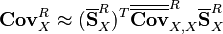
- It applies the Sandwich rule:
- where:
 is the sensitivity vector containing the group sensitivities
 is the covariance matrix containing the group covariances
- where:
- The methodology is described in a related report[11].
- It requires setting the sensitivity calculation parameters. For more information, see the detailed description on sensitivity calculations.
set covlib
set covlib LIB1 [ LIB2 LIB3 ... ]
Sets plain ASCII multi-group covariance data file paths. Input values:
| LIBn | : file paths to multi-group covariance data files in the plain ASCII format (ASCII or binary) |
The syntax of the file containing the covariance data is:
NG E1 ... ENG+1 NM ZAI1,1 MT1,1 ZAI1,2 MT1,2 COV1,1,1 ... COV1,NG,NG ... ZAINM,1 MTNM,1 ZAINM,2 MTNM,2 COVNM,1,1 ... COVNM,NG,NG
where:
| NG | : number of neutron energy groups |
| Eg | : energy grid boundaries [in MeV] |
| NM | : number of covariance matrixes |
| ZAIm,n, MTm,n | : 2 × nuclide (ZAI)-reaction (ENDF reaction MT) pairs defining the m-th covariance matrix |
| COVm,g,g | : NG × NG covariance data corresponding to the m-th matrix |
Notes:
- It enables first-order uncertainty propagation by collapsing the covariance data with the evaluated sensitivities.
- It applies the Sandwich rule:
- It applies the Sandwich rule:
- where: is the sensitivity vector containing the group sensitivities
- is the covariance matrix containing the group covariances
- where:
- The methodology is described in a related report[11].
- It requires setting the sensitivity calculation parameters. For more information, see the detailed description on sensitivity calculations.
set cpd
set cpd DEPTH [ NZ ZMIN ZMAX ] [ LVL1 LVL2 ]
Sets on the calculation of lattice-wise power distributions to output file [input]_core0.m on. Input values:
| DEPTH | : The number of lattice-levels included. |
| NZ | : Number of equal sized axial bins into which the lattices are divided (default value: 1) |
| ZMIN | : Minimum z-coordinate for the axial division [in cm] (default value: -INFTY) |
| ZMAX | : Maximum z-coordinate for the axial division [in cm] (default value: INFTY) |
| LVL1 | : User-defined first level where to define the lattice-wise power distribution |
| LVL2 | : User-defined second level where to define the lattice-wise power distribution |
Notes:
- The interpretation of the number of levels included is as follows:
- DEPTH 1: includes the first level from the root universe, which "usually" corresponds to the assembly-wise distribution.
- DEPTH 2: includes the first two levels from the root universe, which "usually" corresponds to the assembly- and pin-wise distributions.
set cpop
set cpop NPG NGEN NSKIP [ NSKIP2 ]
Sets parameters for simulated neutron population for corrector neutron transport solutions in burnup calculation. Typically used with the SIE burnup scheme. Input values:
| NPG | : number of neutrons per generation |
| NGEN | : number of active generations |
| NSKIP | : number of inactive generations |
| NSKIP2 | : number of inactive generations on further iterations for the same burnup point |
Notes:
- As the SIE burnup scheme executes the corrector step multiple times for each burnup step, combining the results from each iteration, it may be a good idea to run more iterations with less active neutron histories per iteration.
set csw
set csw FILE
Writes source points in criticality source simulation into a file. Input values:
| FILE | : file name where the source points are written |
Notes:
- Only source points from active cycles are included.
- From version 2.2.1 and on, multi-step depletion source files can be generated [FILE]_[bu], where "bu" is the burnup step. Otherwise, simply, [FILE].
set dataout
set dataout TABLE_LIST
Defines the tables included in the nuclear and material data file [input].out. Input values:
| TABLE_LIST | : list of tables (default value: all/0) |
Possible list of tables: Possible key-words/variables are:
Key-word Table ID Description 0, all include all available tables 1, nuc_summary Table 1: Summary of nuclide data 2, nuc_readec Table 2: Reaction and decay data 3, nuc_nfy Table 3: Fission yield data only in burnp mode 4, nuc_lostpath Table 4: Lost transmutation paths only in burnup mode 5, mat_summary Table 1: Summary of material compositions 8, allnuc (nuclide) Tables 1-4 9, allmat (material) Tables 1 -1 omit the [input].out file
Notes:
- The output file data is divided into two sections: nuclear data (Tables 1-4) and material data (Table 1). Respectively, they include all the nuclides and their reactions as they are read from the nuclear data libraries, and the material data includes isotopic compositions and densities, as well as volumes and masses if available.
- For more information, see detailed description of the nuclear and material data output.
set dbrc
set dbrc Emin Emax NUC1 [ NUC2 ... ]
Enables the use of doppler-broadening rejection correction (DBRC). Input values:
| Emin | : Minimum energy for DBRC [in MeV] |
| Emax | : Maximum energy for DBRC [in MeV] |
| NUCn | : zero-kelvin nuclide identifiers for which to apply DBRC (e.g. "92238.00c") |
Notes:
- Use of DBRC requires 0 K cross section data.
- See also Section 5.6 of [1].
- This input could be given without any nuclides before version 2.1.32. Then DBRC was not used at all.
set dd
set dd MODE [ X0 Y0 α0 ]
Invokes domain decomposition. Input values:
| MODE | : decomposition mode (default value: 0) |
| X0 | : x-coordinate of the domain decomposition origin (centre of the radial division, initial position of the angular division) [in cm] (default value: 0.0) |
| Y0 | : y-coordinate of the domain decomposition origin (centre of the radial division, initial position of the angular division) [in cm] (default value: 0.0) |
| α0 | : angular position of the domain decomposition origin [in degrees] (default value: 0.0) |
The possible modes are:
Mode Description Notes 0 none 1 depletion zone indexing-based decomposition not recommended 2 sector-based decomposition X0, Y0 and α0 are available 3 sector-based + central division decomposition X0, Y0 and α0 are available, only applicable if MPI-tasks > 4
Notes:
- Domain decomposition works in MPI mode by separating burnable materials into different parallel tasks.
- The number of domains is given by the number of MPI tasks.
- Only burnable materials separated into depletion zones using the sep entry in the div card are decomposed
- Decomposed materials are plotted in domain-specific colors (unless the rgb entry in the mat card is used)
- The domain decomposition methodology is described in a related paper[12].
- For more information, see the detail description and practical example on the Domain decomposition.
set declib
set declib LIB1 [ LIB2 LIB3 ... ]
Sets the decay data library file paths. Input values:
| LIBn | : library file paths |
Notes:
- Decay libraries are standard ENDF format[3] files containing decay data.
- If the file path contains special characters it is advised to enclose it within quotes.
- A default directory path can be set by defining environment variable SERPENT_DATA. The code looks for decay data files in this path if not found at the absolute.
- From version 2.2.0 and on, a default decay data library directory file can be set by defining environment variable SERPENT_DECLIB.
- This file will be used if no other path is given with set declib.
set decomp
set decomp OPT [ ELEM1 ELEM2 ... ]
Decomposes elemental entries in material cards into isotopes. Input values:
| OPT | : option to include (1) or exclude (0) elements from decomposed list |
| ELEMn | : element names |
Notes:
- Elemental entries are identifed from zero A in ZA.
- The decomposition is based on built-in isotope fractions.
- If the list is not provided, all elemental entries are decomposed.
set delnu
set delnu OPT
Sets delayed neutron emission on or off. Input values:
| OPT | : option to switch delayed neutron emission on (1/yes) or off (0/no) |
Notes:
- Default values:
- Criticality source mode: the delayed neutron emission is "on"
- External (static/dynamic) source mode: the delayed neutron emission is "off"
- In time-dependent calculations, driven by the set dynsrc option, precursor based delayed neutron emission is included in the calculation
- "off" at fission, but "on" at delayed nubar in total nubar.
- See separate description of physics options in Serpent for differences to other codes.
set depmtx
set depmtx MODE
Print burnup matrixes to [input]_depmtx_[mat]_[bu]_[ss].m file during burnup calculation, where "bu" is the burnup step and "ss" is the substep. Input values:
| MODE | : option to switch on (1/yes) or off (0/no) the printing of burnup matrixes. The default value is "off" |
Notes:
- With non-constant predictor, this option will stop the simulation up to version 2.1.31.
- With multiple substeps, only the last one is kept after the simulation up to version 2.1.31.
- The burnup matrix output is named depmtx_[mat][bu].m up to version 2.1.31.
set depout
set depout MODE [STEP]
Controls which burnable material compositions are printed into the binary [input].dep and plain text [input]_dep.m depletion output files in case of divided materials. Input values:
| MODE | : value indicating, which materials to output to the [input].dep and [input]_dep.m files (1 = only partials, 2 = only parents, 3 = both). (default value: 2) |
| STEP | : value indicating the print-out interval of the [input]_dep.m file (0 = final step, 1 = all steps, 2 = none). (default value: 1) |
Notes:
- Parent materials refer to materials defined by mat cards, and partials to depletion zones created automatically using the div card.
- If the post-processing re-depletion -rdep command line option is desired to print the partial material output (MODE value 1 or 3), the respective MODE value has to be present in the original depletion calculation.
- Print-out interval step option 2 (no [input]_dep.m generation) can be combined with the above-mentioned post-processing re-depletion to suppress the plain text output during the original depletion calculation.
- Combined with the domain decomposition feature (set dd option):
- If the mode is different from 2, it generates multiple depletion files which are named adding _dd[mpiid] (domain decomposition identifier) to the standard file name.
- Each of them contains the partial materials information of the given domain/MPI task.
set deppara
set deppara PARAM_LIST
Defines the material- and isotopic-wise variables included in the depletion output file [input]_dep.m. Input values:
| PARAM_LIST | : list of variables (default value: "all") |
Possible key-words/variables are:
Key-word Quantity Output ID Description atom atom density ADENS [in b-1cm-1] mass mass density MDENS [in g/cm3] activity activity A [in Bq] dh decay heat H [in W] sf spontaneous fission rate SF [in fissions/s] gsrc photon emission rate GSRC [in photons/s] ingtox ingestion toxicity ING_TOX [in Sv] inhtox inhalation toxicity INH_TOX [in Sv] all include full-set of variables none exclude full-set of variables
Notes:
- For more information, see detailed description of the burnup calculation output.
set depstepbunorm
set depstepbunorm NORM
Sets the depletion step normalization in burnup calculations based on energy deposition. Input values:
| NORM | : depletion step normalization mode based on energy deposition (1 = all materials, 2 = burnable materials) |
Notes
- Default values (see set edepmode):
- For energy deposition modes 0/1: the normalization includes only "burnable" materials - mode 2.
- For energy deposition modes 2/3: the normalization includes "all materials" - mode 1.
set dfsol
set dfsol MODE [ DC NP ]
Options for homogeneous diffusion flux solver. Input values:
| MODE | : boundary conditions for solver (1 = include net currents at boundary surfaces and corners, 2 = include only surface currents). (default value: 1) |
| DC | : type of diffusion coefficient used in the calculation (1 = out-scattering 2 = transport correction). (default value: 1) |
| NP | : number of points for trapezoidal integration for homogeneous flux (default value: 100) |
Notes:
- This input option is used to control how the deterministic diffusion flux solver used to obtain assembly discontinuity factors (set adf) and pin power distributions (set ppw) is run.
- The option syntax was revised in update 2.1.27 (DC option was added between MODE and NP).
- Deterministic diffusion flux solver use:
- Out-scattering approximation, INF_DIFFCOEF and INF_TRANSPXS.
- Transport correction, TRC_DIFFCOEF and TRC_TRANSPXS. It requires enabling the set trc option.
- For more information, see a detailed description on the built-in diffusion flux solver.
set dix
set dix OPT
Sets double indexing for cross section energy grid look-up on or off. Input values:
| MODE | : option to set double indexing on (1/yes) or off (0/no) |
Notes:
- Double indexing is a method to speed-up the cross section look-up when energy grid unionization is not used for microscopic data.
- The method can be used only in optimization modes 1 and 3 (modes 2 and 4 are based on energy grid unionization), see set opti option.
- The methodology is described in related paper[13]
set dspec
set dspec EGRIDp EGRIDn
Sets the energy grid structure for decay spectra. Input values:
| EGRIDp | : energy grid structure for photons |
| EGRIDn | : energy grid structure for neutrons |
Notes:
- The photon/neutron decay spectra is printed in the [input]_gsrc.m or [input]_nsrc.m output file, respectively.
- The energy group spectra only include the contribution from the discrete/line spectra.
- There is a special entry for the energy grid structure, EGRID:
- "-1": instead of providing the energy grid structure, it disables the option for the given particle type.
set dt
set dt NTRSH [ GTRSH ]
Sets probability threshold for delta-tracking. Input values:
| NTRSH | : probability threshold for neutrons (default value: 0.9) |
| GTRSH | : probability threshold for photons (default value: 0.9) |
Notes:
- Tracking algorithm mode:
- Delta-tracking is used by default for both neutrons and photons
- Switch to surface-tracking happens if the probability of sampling virtual collisions (ratio between material total cross section and the majorant) exceeds the given threshold.
- Probability threshold:
- The default probability threshold for both particle types is 0.9: i.e. delta-tracking is used if the ratio between total cross section and majorant is above 0.1.
- To enforce delta-tracking mode always: use "1".
- To enforce surface-tracking mode always: use "0"
- Use of delta-tracking can be enforced or blocked in individual materials using the set forcedt and set blockdt options
- Integral reaction rates are scored using the collision estimator of neutron flux, which has a few adjustable parameters (see set cfe option).
- For more information on tracking modes, see the detailed description on delta- and surface-tracking.
set dynccfile
set dynccfile OPT
Option to store precursors and neutrons between time steps in coupled dynamic simulations into a file. Input values:
| OPT | : option to switch on (1/yes) or off (0/no) the store/write dynamic data into a file. The default option is "on". |
set dynsrc
set dynsrc PATH [ MODE ]
Links previously generated steady state source distributions to be used in a transient simulation with delayed neutron emission. Input values:
| PATH | : The path of the previously generated source file (without the .main suffix) |
| MODE | : Precursor tracking mode (0 = mesh based, 1 = point-wise) |
Notes:
- Four source files will be required [PATH].main, [PATH].prec, [PATH].live and [PATH].precpoints
set ecut
set ecut EMINn [ EMINp ]
Sets minimum energy cut-off for neutrons and photons. Input values:
| EMINn | : cut-off energy for neutrons [in MeV] (default value: -INFTY/"no cut-off") |
| EMINp | : cut-off energy for photons [in MeV] (default value: 1.0E-3) |
Notes:
- Using energy cut-off for neutrons may lead to non-physical results, since fission and up-scattering may not be accurately modeled.
- Versions 2.1.27 and earlier include only photon energy cut-off, which is now the second input parameter.
set ecutdens
set ecutdens DENS1 EMINp,1 [ DENS2 EMINp,2 ... ]
Sets density-wise minimum energy cut-off for photons. Input values:
| DENSi | : mass density [in g/cm3] |
| EMINp,i | : cut-off energy for photons [in MeV] |
Notes:
- Mass densities and energy cut-offs must be given in ascending order.
set ecutmat
set ecutmat MAT1 EMINp,1 [ MAT2 EMINp,2 ... ]
Sets material-wise minimum energy cut-off for photons. Input values:
| MATi | : material name |
| EMINp,i | : cut-off energy for photons [in MeV] |
set eddi
set eddi OPT
Option that enables the calculation of Eddington factors. Input values:
| OPT | : option to switch calculation on (1/yes) or off (0/no). The default option is "off". |
Notes:
- Requires group constant generation to be set on (see set gcu).
set edepdel
set edepdel OPT [ LOCAL_EGD ]
Option to include the energy of delayed components in energy deposition calculations. Input values:
| OPT | : include (1/yes) or exclude (0/no) the energy of delayed components in energy deposition estimates (default value: 1) |
| LOCAL_EGD | : deposit the energy of the delayed fission gammas to fission sites (1) or with the same distribution as the prompt fission gammas (0). (default value: 0) |
Notes:
- Delayed components include delayed neutrons, delayed fission gammas and delayed betas.
- The energy of the delayed components is deposited at the time of fission so the time dependence of the energy deposition is not accounted for properly in transient simulations.
- The energy of delayed neutrons can be excluded using this option only in energy deposition mode "1" (see set edepmode option).
- Option to deposit the energy of the delayed fission gammas with the same distribution as the prompt fission gammas (LOCAL_EGD = 0) does not work in external source simulations and if it is used the energy of the delayed fission gammas is not accounted for.
set edepkcorr
set edepkcorr OPT
Option to apply correction for energy deposition estimates when simulating non-critical systems with criticality source mode. Input values:
| OPT | : option to switch the correction on (1/yes) or off (0/no). The default option is "on". |
Notes:
- The methodology is described in related paper. [14]
set edepmode
set edepmode MODE [ E_CAPT ]
Sets energy deposition mode for energy deposition calculations. Input values:
| MODE | : energy deposition mode: 0, 1, 2 or 3 (default value: 0) |
| E_CAPT | : additional energy release in capture reactions given [in MeVs per fission] (default value: 0.0) |
The possible setting for mode are:
Mode Description Evaluation 0 Constant energy deposition per fission Efiss,i = (Qi/Q235) × H235 1 Local energy deposition based on ENDF MT 458 data Efiss,i = EFRi + ENPi + ENDi + EGPi + EGDi + EBi + Ecapt 2 Local photon energy deposition Efiss,i = EFRi + EGPi + EGDi + EBi 3 Coupled neutron-photon transport Efiss,i = EFRi + EBi
Notes:
- The energy deposition modes are described in related paper [14] which also includes some discussion on the problems in the data used by the energy deposition modes.
- The additional energy release in capture reactions is only used in energy deposition mode "1"
- The choice of energy deposition mode affects also the normalization of the results, if normalization to total power or power density is used.
- Energy deposition modes "1", "2" and "3" require data which is not available in the standard ACE-format cross section files used by Serpent. Separately distributed ACE-files (file endfb71_edep.tar.gz) containing additional data are required to use these modes.
- KERMA coefficients used in energy deposition modes "2" and "3" are not Doppler-broadened correctly by the built-in preprocessor. See Doppler-broadening preprocessor.
- The energy deposition modes "1", "2" and "3" have been tested mainly in criticality source simulations and one should proceed with caution when using them in other types of calculations such as transient and burnup calculations.
set egrid
set egrid TOL [ EMIN EMAX ]
Sets the unionized energy grid reconstruction parameters. Input values:
| TOL | : fractional reconstruction tolerance |
| EMIN | : minimum energy in the grid [in MeV] |
| EMAX | : maximum energy in the grid [in MeV] |
Notes:
- Default values:
- Fraction reconstruction tolerance: 0.0 (transport calculation mode), 5.0E-05 (burnup calculation mode)
- Energy grid boundaries: [1.0E-11, 20.0] (neutrons), [1.0E-03, 100.0] (photons)
- A higher energy grid reconstruction tolerance means lower memory consumption and possibly higher computation speed but also reduced accuracy of the calculation.
- See also Section 5.3 of [1].
set ekn
set ekn E
Sets the Klein-Nishina equation to approximate a Compton scattering event. Input values:
| E | : energy cut-off for modelling energy and direction of the scattered photon [in MeV] (default value: INFTY/"no cut-off") |
Notes:
- The Klein-Nishina equation is used above E for calculating both the energy and direction of the scattered photon. Below E, the Doppler brodening method is used if switched on. Otherwise, the incoherent scattering function approximation is in use.
- The photon transport physics model is described in a related paper[6]
set elcond
set elcond MAT1 COND1 [ MAT2 COND2 ... ]
Sets material-wise conductivity state for electrons in photon transport calculations. Input values:
| MATi | : material name |
| CONDi | : conductivity state (0 = non-conductor, 1 = conductor, 2 = conduction electron dependent). (default value: 2) |
Notes:
- If the material is set as a conductor and no-conduction electrons are found, the material conductivity state is overwritten to non-conductor.
- For conductivity state 2, conduction electron dependent, establishes that a single element material is a conductor if conduction electrons are found, otherwise is a non-conductor. A compound is always a non-conductor.
set elgas
set elgas MAT1 GAS1 [ MAT2 GAS2 ... ]
Sets material-wise phase for electrons in photon transport calculations. Input options:
| MATi | : material name |
| GASi | : phase state (0 = condensed or non-gas, 1 = gas). (default value: 0) |
Notes:
- The default option "0/condensed" only affects mixtures.
- The gas phase does not affect the mean excitation energy of a single material: if set elmee option is set for a material, the material is considered as non-gas.
set elmee
set elmee MAT1 MEE1 [ MAT2 MEE2 ... ]
Sets material-wise mean excitation energy for electrons in photon transport calculations. Input values:
| MATi | : material name |
| MEEi | : electrons mean excitation energy [in MeV] (default value: -1) |
Notes:
- There is a special entry for the MEEi parameter:
- "-1": mean excitation energy calculated during runtime for compounds and extracted from data for single element materials.
- The maximum mean excitation energy for electrons is 1 MeV.
set elspn
set elspn EGRID_E
Sets the stopping power energy grid size for electrons/positrons in photon transport calculations. Input values:
| EGRID_E | : energy grid size (default value: 200) |
Notes:
- The thick-target bremsstrahlung model (see set ttb option) assumes that the energy array is uniformly distributed in a log-energy scale.
set entr
set entr NX NY NZ [ XMIN XMAX YMIN YMAX ZMIN ZMAX ]
Defines the mesh structure used for calculating fission source entropy. Input values:
| NX | : number of mesh cells in x-direction (default value: 5) |
| NY | : number of mesh cells in y-direction (default value: 5) |
| NZ | : number of mesh cells in z-direction (default value: 5) |
| XMIN | : minimum mesh boundary in x-direction [in cm] |
| XMAX | : maximum mesh boundary in x-direction [in cm] |
| YMIN | : minimum mesh boundary in y-direction [in cm] |
| YMAX | : maximum mesh boundary in y-direction [in cm] |
| ZMIN | : minimum mesh boundary in z-direction [in cm] |
| ZMAX | : maximum mesh boundary in z-direction [in cm] |
Notes:
- Shannon entropy is used to monitor fission source convergence, in criticality source simulations.
- For more information, see detailed description on fission source convergence.
- The calculation is invoked by setting the generation history record option on the set his option.
- It records the distribution of source points on mesh: [input]_his[n].m, where "n" is the burnup index.
- For more information, see detailed description on the History output.
- If no mesh boundaries are specified, the mesh extends over the entire geometry.
set fininitfile
set fininitfile FILEPATH
Links a file containing an initial fuel behavior solution used as a starting point for a coupled calculation with the FINIX fuel behavior module. Input values:
| FILEPATH | : path to the file |
Notes:
- The file should be a type 6 fuel behavior interface containing a previous solution from a coupled FINIX calculation.
- The axial and radial nodalization as well as the included fuel rods should be the same in the file as in the calculation.
set fissh
set fissh ZAI1 E1 ZAI2 E2 ...
Overrides default fission heating values. Input values:
| ZAIn | : nuclide identifiers (ZAI) |
| En | : energy deposited per fission [in MeV] (default value: 202.27) |
Notes:
- The energy deposited per fission includes additional energy released in capture reactions when fission neutrons are absorbed.
- The energy release per fission value for other actinides is scaled based the Q-values found in the cross section libraries in reference with the U-235 value set.
- See also set U235H option.
- See also Section 5.8 of [1].
set fissrate
set fissrate F [ MAT ]
Sets normalization to fission rate. Input values:
| F | : number of fission reactions per second [in 1/s] |
| MAT | : dummy parameter |
Notes:
- Normalization is needed to relate the Monte Carlo reaction rate estimates to a user-given parameter.
- The default normalization:
- It is set to unit total loss rate (neutron transport) and to unit total source rate (photon transport).
- In coupled neutron-photon transport simulations the normalization is driven by the neutron normalization
- For other normalization options, see: set power, set powdens, set flux, set genrate, set absrate, set lossrate, set srcrate, set sfrate.
- If multiple depletion histories and normalizations are defined in the input, the first normalization will be used with the first depletion history, the second normalization with the second depletion history and so on.
- See also Section 5.8 of [1].
set fissye
set fissye INTT
Sets the energy-dependent interpolation scheme for the fission yields. Input values:
| INTT | : energy-dependent interpolation (0 = none, 1 = linear-linear, 2 = histogram). The default option is "1/linear-linear". |
Notes:
- The default option "1/linear-linear" is based on the two-dimensional interpolation scheme dictated by the ENDF data (File 8: Decay and Fission Product Yields - sec. 0.5.2.2)[3].
- The interpolation is defined by the neutron energy spectrum.
- The option "0/none" excludes the energy-dependency from the fission yields, i.e. single-value defined at the lower limit.
- The option "2/histogram" implies that the function is constant and equal to the value given at the lower limit of the interval (e.g., thermal, epithermal, fast values).
- It is defined in connection with how the data were measured in thermal and fast systems. (Note that the option is under evaluation).
set flux
set flux F [ MAT ]
Sets normalization to total flux. Input values:
| F | : flux |
| MAT | : dummy parameter |
Notes:
- Normalization is needed to relate the Monte Carlo reaction rate estimates to a user-given parameter.
- The default normalization:
- It is set to unit total loss rate (neutron transport) and to unit total source rate (photon transport).
- In coupled neutron-photon transport simulations the normalization is driven by the neutron normalization.
- For other normalization options, see: set power, set powdens, set genrate, set fissrate, set absrate, set lossrate, set srcrate, set sfrate.
- If multiple depletion histories and normalizations are defined in the input, the first normalization will be used with the first depletion history, the second normalization with the second depletion history and so on.
- See also Section 5.8 of [1].
set fluxlimtrc
set fluxlimtrc OPT
Option that enables the calculation of flux limited TRC diffusion coefficients. Input values:
| OPT | : option to switch calculation on (1/yes) or off (0/no). The default option is "off". |
Notes:
- In infinite-spectrum calculations the anisotropic component of the non-TRC nuclides/materials is removed
- S1 and SP1 are non-corrected for non-TRC nuclides/materials and below energy limit for TRC nuclides/materials (see set trc option)
set fmtx
set fmtx 1 MAT1 MAT2 ...
set fmtx 2 UNI1 UNI2 ...
set fmtx 3 LVL
set fmtx 4 XMIN XMAX NX YMIN YMAX NY ZMIN ZMAX NZ
Set the calculation of fission matrixes. Input values:
| MATn | : material list |
| UNIn | : universe list |
| LVL | : level number |
| XMIN | : minimum x-coordinate mesh boundary [in cm] |
| XMAX | : maximum x-coordinate mesh boundary [in cm] |
| NX | : number of x-mesh cells |
| YMIN | : minimum y-coordinate mesh boundary [in cm] |
| YMAX | : maximum y-coordinate mesh boundary [in cm] |
| NY | : number of y-mesh cells |
| ZMIN | : minimum z-coordinate mesh boundary [in cm] |
| ZMAX | : maximum z-coordinate mesh boundary [in cm] |
| NZ | : number of z-mesh cells |
Notes:
- There are four options for defining the regions that compose the matrix: 1 = material, 2 = universe, 3 = level, 4 = Cartesian mesh.
- Output values are given in pairs: matrix element and associated relative error, for total, prompt and delayed (analog) fission matrixes.
- The output is printed in file [input]_fmtx[bu].m, where "bu" is the burnup step.
set forcedt
set forcedt MAT1 MAT2 ...
Defines the list of materials where delta-tracking is always used. Input values:
| MATn | : material names |
Notes:
- This option is used to override selection of tracking mode based on the probability threshold (see set dt option) in individual materials.
- Use of delta-tracking can be blocked in individual materials using set blockdt option.
- For more information on tracking modes, see the detailed description on delta- and surface-tracking.
- Note to developers: should have different lists for neutrons and photons?
set fpcut
set fpcut FPCUT
Sets the fission product yield cut-off. Input values:
| FPCUT | : fission product yield cut-off (default value: 0.0) |
Notes:
- Fission product yield cut-off acts on cumulative fission yields.
- The FPCUT parameter represents the lower limit for the maximum cumulative yield in each mass chain.
- For example, a value of "1E-2" means that every mass chain (nuclides with same mass number) with all cumulative yields below 1% are discarded from the calculation.
- Setting the cut-off to a higher value (~1E-4 or so) is an effective way to reduce the number of nuclides in the calculation, but at some point it will start affecting the results.
set fsp
set fsp OPT NSKIP
Sets fission source passing between two transport simulations in burnup or coupled calculation. Input values:
| OPT | : option to switch fission source passing on (1/yes) or off (0/no). The default option is "off". |
| NSKIP | : number of inactive generations on subsequent steps |
Notes:
- The fission source at the end of one transport calculation is used as the initial source for the next transport calculation.
- Number of inactive generations is taken from set pop option on the first step and from set fsp option on all later steps.
set fum
set fum ERG [ BTCH MODE LIM ]
set fum ERG [ BTCH MODE LIM TGT ITER INIT ]
set fum ERG [ BTCH MODE DC LIM TGT ITER INIT ]
Activates fundamental mode calculation for collapsing intermediate multi-group constant data into few-group constants with a critical spectrum. Input values:
| ERG | : Intermediate multi-group structure for calculation of the leakage-corrected critical spectrum (default value: Default multi-group structure, 70 energy-groups) |
| BTCH | : Micro-group batching option (1 = cycle-wise, 2 = averaged over all criticality cycles) |
| MODE | : Critical spectrum calculation mode (default value: 0) |
| DC | : Multi-group diffusion coefficients scheme to be used only with MODE = 3 (default value: 1 = out scattering). |
| LIM | : Convergence criterion of keff, evaluated as the absolute value difference of keff between successive iterations, with MODE = 1, 2, 3 (default value: 1E-7) |
| TGT | : Target value for keff with MODE = 1, 2, 3 (default value: 1.0) |
| ITER | : Maximum number of fundamental mode calculation iterations, with MODE = 1, 2, 3 (default value: 25) |
| INIT | : First guess for absolute value of critical B2, with MODE = 1, 2, 3 (default value: 1E-6) |
The possible values for mode are:
Mode Description o, O, 0 Old B1 calculation (use the same method as before version 2.1.31) b, B, 1 New B1 calculation p, P, 2 P1 calculation f, F, 3 FM calculation
The possible values for FM mode multi-group diffusion coefficients are:
Notes:
- It invokes the calculation of leakage corrected flux: critical flux, on group constants and produces an additional set of homogenenized group constants ("B1_").
- The output prefix "B1_" is invariant, regardless of the critical spectrum calculation mode.
- The B1 group constant estimates are written in:
- [input]_res.m output file: group constants homogenized in leakage-corrected spectrum sub-section
- [input].coe ouput file, via the set coefpara option: automated burnup sequence/coefficient matrix output.
- Intermediate group structure:
- The multi-group structure may be an energy grid defined using the ene card or a name of a pre-defined energy group structure.
- Setting the FM calculation overrides the default 70-group structure used for macroscopic data calculation in infinite spectrum.
- In general the intermediate multi-group structure should have more groups than the few-group structure to get reasonable results for leakage corrected group constants and out-scatter diffusion coefficients.
- Averaging the results over all cycles, BTCH = 2, may improve convergence and speed up the calculation, but all information on statistical errors is lost.
- Calculation modes:
- Before version 2.1.31, the MODE parameter was not read, and the old B1 calculation mode was always used regardless of the parameter given here.
- The calculation modes other than the old B1 calculation mode were added in version 2.1.31.
- Mode 0 (old B1 calculation) might be very slow with a large intermediate multi-group structure (for example with approximately 2000 groups). Modes 1-3 should run much faster.
- Limitations:
- The leakage correction option does not affect the flux spectrum used during burnup calculations.
- Alternatively, use the implicit leakage correction via MC-Fundamental Mode (see set mcleak option), where the all estimates are leakage corrected.
- The set fum and set mcleak options are mutually exclusive.
- The leakage correction option does not affect the flux spectrum used during burnup calculations.
set gbuf
set gbuf FAC [ BNK ]
Sets the size of photon buffer and event bank. Input values:
| FAC | : factor (> 1) defining the buffer size |
| BNK | : event bank size |
Notes:
- Photon buffer refers to pre-allocated memory block used to store photon particle data.
- This memory is needed for putting secondary photons in que, etc..
- The buffer factor FAC defines the buffer size relative to simulated batch size.
- The event bank BNK refers to pre-allocated memory block used to store history data on particle events.
- This bank is used only with certain special options, such as importance detectors and track plotter.
- The default values depend on simulation mode, and there is no need to adjust the values unless the calculation terminates with an error.
- Note to developers: event bank is now the same for both neutrons and photons.
set gct
set gct OPT
Option that enables the calculation of group constant statistics tests. Input values:
| OPT | : option to switch calculation on (1/yes) or off (0/no). The default option is "off". |
Notes:
- When this option is set, the batch-wise statistical tests are printed in the file [input]_stat.m.
- Requires group constant generation to be set on (see set gcu option).
- For more information:
- Note to developers: statistical tests should be documented
set gcu
set gcu UNI1 [ UNI2 UNI3 ... ]
Sets the universes for group constant generation. Input values:
| UNIn | : universe where group constants are generated (default value: 0 = root universe) |
Notes:
- By default, group constants are generated in the root universe.
- Super-imposed group constant generation universes (i.e. not part of the geometry definition) should not be used so that they cover (partly or totally) the same geometry region as some other group constant generation universe (super-imposed or part of the geometry definition), if group constants are generated only on a single geometry level.
- There is a special for the UNI1 entry:
- "-1": to switch the group constant generation "off" (single entry)
- The group constant generation should be switched "off" when the results are not needed (this may speed up the calculation).
- Note that this will also disable e.g. writing of the [input].coe ouput file.
- The homogenized group constant parameters are written in
- [input]_res.m file (by default): homogenized group constants section.
- [input].coe ouput file, via the set coefpara option: automated burnup sequence/coefficient matrix output.
- The spatial homogenization methodology is described in a related paper[16].
set gcut
set gcut GMAX
Sets generation cut-off for neutrons. Input values:
| gmax | : number of simulated generations before cut-off |
Notes:
- The generation cut-off can be used in neutron external source simulations, to limit the length of fission chains.
- Applicable only to neutron external source simulation (invoked using set nps option)
- Generation or time cut-off (see set tcut option) is always needed for neutron external source simulations in super-critical systems.
set genrate
set genrate G [ MAT ]
Sets normalization to fission neutron generation rate. Input values:
| G | : number of fission neutrons emitted per second [in neutrons/s] |
| MAT | : material in which the fission neutrons are generated. The default is all materials |
Notes:
- Normalization is needed to relate the Monte Carlo reaction rate estimates to a user-given parameter.
- If the material name is omitted, the value corresponds to total fission neutron generation rate in the system.
- The neutron generation rate includes only prompt and delayed neutrons emitted in fission.
- The default normalization:
- It is set to unit total loss rate (neutron transport) and to unit total source rate (photon transport).
- In coupled neutron-photon transport simulations the normalization is driven by the neutron normalization.
- For other normalization options, see: set power, set powdens, set flux, set fissrate, set absrate, set lossrate, set srcrate, set sfrate.
- If multiple depletion histories and normalizations are defined in the input, the first normalization will be used with the first depletion history, the second normalization with the second depletion history and so on.
- See also Section 5.8 of [1].
set gpop
set gpop MAX_HIS MAX_POP C
Sets the on-the-fly neutron growing population size algorithm. Input values:
| MAX_HIS | : maximum number of histories |
| MAX_POP | : maximum population size |
| C | : parameter to control the population growth |
Notes:
- The on-the-fly neutron growing population size algorithm is used in criticality calculations to accelerate the fission source convergence.
- The growing algorithm methodology is described in related paper. [17]
set gsw
set gsw FILE [ OPT ]
Writes secondary photon source points in coupled neutron-photon transport simulation into a file. Input values:
| FILE | : file name where the source points are written |
| OPT | : option to include (1/yes) or exclude (0/no) secondary photons in transport calculation. The default option is "off". |
Notes:
- Applicable only to coupled neutron-photon transport simulation (invoked using set ngamma).
- Only source points from active cycles are included in criticality source simulations.
- From version 2.2.1 and on, multi-step depletion source files can be generated [FILE]_[bu], where "bu" is the burnup step. Otherwise, simply, [FILE].
set his
set his OPT
Sets batch history record on or off. Input values:
| OPT | : option to switch batch history record on (1/yes) or off (0/no). The default option is "off". |
Notes:
- When invoked, Serpent collects batch-wise data on keff, fission source entropy etc. and produces a separate file: [input]_his[n].m
- For more information, see the description of the history output.
- Setting the history option also invokes the calculation of fission source (Shannon) entropy.
- The entropy mesh parameters can be adjusted using set entr option.
set ifp
set ifp GEN
Sets the number of generations to use for calculating the iterated fission probability. Input values:
| GEN | : Number of generations (default value: 15). |
set imp
set imp TYPE G
Defines energy-dependent importances. Input values:
| TYPE | : type of dependency (e = energy) |
| G | : exponential for adjusting importances (default value: -0.5) |
set imp TYPE r1 I1 [ r2 I2 ... ]
Defines geometry-dependent importances for given region(s). Input values:
| TYPE | : type of (geometrical) dependency (c = cell, m = material, u = universe) |
| rn | : region identifier (cell, material or universe name) |
| In | : importance |
Notes:
- Geometry-dependent importances (only) used for variance reduction
- Only cell (geometry-dependent) type importances supported for now
- Geometry-dependent importances requires using surface-tracking (see set dt)
set impl
set impl ICAPT [ INXN INUBAR ILEAK ]
Sets implicit reaction modes on or off. Input values:
| ICAPT | : option to switch implicit capture reactions on (1/yes) or off (0/no) |
| INXN | : option to switch implicit nxn reactions on (1/yes) or off (0/no) |
| INUBAR | : number of fission neutrons to emit in each fission (nonzero = implicit treatment, 0 = analog treatment) |
| ILEAK | : option to switch implicit implicit leakage on (1/yes) or off (0/no) |
Notes:
- Group constant generation (see set gcu option) requires implicit nxn reactions to be set "on".
- If an implicit nubar is given, the weights of the fission neutrons are scaled to conserve the physical number of fission neutrons.
- Implicit leakage requires group constant generation (see set gcu option) to be set "on".
- See separate description of physics options in Serpent for differences to other codes.
set inftrk
set inftrk LOOPn [ ERRn LOOPp ERRp ]
Sets parameters for terminating infinite tracking loops. Input values:
| LOOPn | : number of neutron tracking loops interpreted as a geometry error (default value 1E6) |
| ERRn | : flag to terminate neutron tracking when an infinite loop occurs: on (0/no) or off (1/ yes). The default option is "on" |
| LOOPp | : number of photon tracking loops interpreted as a geometry error (default value 1E6) |
| ERRp | : flag to terminate photon tracking when an infinite loop occurs: on (0/no) or off (1/ yes). The default option is "on" |
Notes:
- Serpent checks for tracking loop length to avoid simulation being stuck in an infinite loop.
- Long loops can occur by chance in complicated geometries, and this parameter allows continuing the simulation without terminating with error message.
- Even if the problem can be solved by switching the infinite loop error "off", it is advised to check the geometry for possible errors.
set inventory
set inventory ID1 ID2 ...
Defines the nuclides or elements to include in the depletion output file [input]_dep.m. Input values:
| IDn | : Identifier for nuclide, or element or special entry. |
Notes:
- Besides the nuclides or elements specified, the output includes the sum over all isotopes.
- Nuclides are entered using element symbol and mass number (e.g U-235, Am-242m, etc.) or ZAI (922350, 952421, etc.).
- In the ZAI format the last digit refers to the isomeric state (0 = ground state, 1 = isomeric state).
- For more information, see the detailed description on Nuclide IDs
- Elements are entered using symbol or numerical (U, 92, etc.).
- Special entries include:
Key-word Description all all nuclides accident nuclides with significant health impact & high migration probability in accident conditions[18] actinides actinides (Z>88) for which cross section data are found in JEFF-3.1.1 burnupcredit nuclides commonly considered in burnup credit criticality analyses for PWR fuels [19] burnupindicators burnup indicators (commonly measured from spent fuel) [19] cosi6 inventory list used by the COSI6 code (excluding lumped fission products) lanthanides lanthanides (56<Z<72) for which cross section data are found in JEFF-3.1.1 longterm relevant radionuclides in long-term waste analyses [20] minoractinides minor actinides (actinides - thorium - uranium - plutonium) for which cross section data are found in JEFF-3.1.1 fp fission products dp actinide decay products (from Serpent 1) ng noble gases
- The detailed list of nuclides associated with each special entry: Pre-defined inventory lists
set inventory top N PARA
Defines the criterion or variable based on which to include the most significant contributors under that category in the depletion output file [input]_dep.m. Input values:
| N | : Number of nuclides |
| PARAM | : Parameter name |
Notes:
- The contribution criterion is based on the variables evaluated in the depletion calculation and outputted in the bunurp output.
- The possible key-words/variables are:
Key-word Description mass contribution to mass fraction activity contribution to activity dh contribution to decay heat sf contribution to spontaneous fission rate gsrc contribution to gamma emission rate ingtox contribution to ingestion toxicity inhtox contribution to inhalation toxicity
- For example: "top 10 dh" gives the top 10 contributors to decay heat.
- The special entries and the calculation of top contributors do not work with the re-depletion -rdep command line option.
set isobra
set isobra ZAI1 MT1 FG1
           ZAI2 MT2 FG2
           ...
Defines constant branching ratios to isomeric states. Input values:
| ZAIn | : nuclide identifiers (ZAI) |
| MTn | : reaction identifiers (ENDF reaction MT) |
| FGn | : fraction of reactions leading to the ground state of the product nuclide |
Notes:
- Serpent uses constant branching ratios by default. This option overrides the default values.
- Energy-dependent data read read from ENDF format[3] files defined by the set bralib option overrides the constant ratios.
set iter alb
set iter alb [ CYCLES KEFF FX FY FZ ]
Option that iterates the albedo boundary conditions given a target k-eff for the evaluation. Input values:
| CYCLES | : number of additional inactive cycles to run for the convergence of the iteration (default value: 50) |
| KEFF | : target keff for the iteration (default value: 1.0) |
| FX | : albedo factor in x-direction to normalize the albedo leakage rate (default value: 1.0) |
| FY | : albedo factor in y-direction to normalize the albedo leakage rate (default value: 1.0) |
| FZ | : albedo factor in z-direction to normalize the albedo leakage rate (default value: 1.0) |
Notes:
- The albedo boundary conditions result from the product of the iterated albedo leakage rate by the albedo factor in each direction.
set iter nuc
set iter nuc CYCLES KEFF NZAI ZAI1 ZAI2 ... ZAINZAI [ NMAT MAT1 MAT2 ... MAXNMAT ]
| CYCLES | : number of additional inactive cycles to run for the convergence of the iteration |
| KEFF | : target keff for the iteration |
| NZAI | : number of different nuclides (ZAI) included in the iteration |
| ZAIi | : the ZAI of the nuclide to be included in the iteration (e.g. 50100 for boron 10 ground state) |
| NMAT | : number of different materials included in the iteration (optional parameter) |
| MATi | : the name of the material to be included in the iteration |
Notes:
- If a list of materials is not given, all materials that contain the included nuclides are included in the iteration.
- The initial density of the nuclides to be iterated should be larger than zero.
- The critical density iteration only works for nuclides that have a reactivity effect mainly through neutron absorption.
- Specifically, critical densities of fissile, moderating or reflecting nuclides cannot be reliably iterated using this card.
- The atomic density of the nuclides is updated according to the batching interval set in the set pop option.
- Having a large batching interval means that the atomic density may take a large number of cycles to converge.
- For more information, see the detailed description on the Critical density iteration.
set keff
set keff KEFF
Option to scale fission neutron production in external source simulations. Input values:
| KEFF | : Fission neutron production scaling factor (default value: 1.0) |
Notes:
- The k-effective to use for scaling the fission neutron production.
- The inverse of KEFF is used as a multiplicative constant for the nubar, i.e. a value of 2.0 will cut the fission neutron production in half.
- The option affects both prompt and delayed neutron production from fissions.
- In versions prior to 2.1.31, it does not affect delayed neutron precursor production, which cases unexpected an behaviour in Transient simulations that track delayed neutron precursor concentrations.
set lossrate
set lossrate L [ MAT ]
Sets normalization to total loss rate. Input values:
| L | : number of lost neutrons per second [in neutrons/s] |
| MAT | : dummy parameter |
Notes:
- Normalization is needed to relate the Monte Carlo reaction rate estimates to a user-given parameter.
- Loss rate includes absorption rate and leakage.
- The default normalization:
- It is set to unit total loss rate (neutron transport) and to unit total source rate (photon transport).
- In coupled neutron-photon transport simulations the normalization is driven by the neutron normalization.
- For other normalization options, see: set power, set powdens, set flux, set genrate, set fissrate, set absrate, set srcrate, set sfrate.
- If multiple depletion histories and normalizations are defined in the input, the first normalization will be used with the first depletion history, the second normalization with the second depletion history and so on.
- See also Section 5.8 of [1].
set lost
set lost LIM
Option to treat undefined geometry regions as void. Input values:
| LIM | : maximum number of collisions allowed in undefined regions (default value: 0) |
Notes:
- This option allows the calculation to proceed even if the geometry routine encounters undefined cells.
- The option is intended, for example, for complex geometries in which the boundaries of adjacent cells may not fully coincide.
- There is a special entry for the number of collisions allowed::
- "-1": if no limit is set
- When the option is set, the number of lost particles is printed in variable LOST_PARTICLES in the [input]_res.m output file.
- The option should not be used to get away with errors in incomplete or poorly defined geometries.
set maxsplit
set maxsplit MAX MIN
Sets limiting values for splitting and Russian roulette. Input values:
| MAX | : maximum number of splits (default value: 1.0E4) |
| MIN | : minimum survival probability in Russian roulette (default value: 1.0E-18) |
Notes:
- It is used with weight-windows (see wwgen card).
set mbtch
set mbtch N
Adjusts the batch used with MPI data transfer. Input values:
| N | : batch size in double floats, i.e. 8 bytes (default value: 1E4) |
Notes:
- The batch size determines the division of data blocks in MPI data transfer.
- The value may have some effect on parallel performance.
set mcleak
set mcleak OPT [ ERG ]
Option that enables the implicit leakage correction via MC-Fundamental Mode. Input values:
| OPT | : option to switch the calculation on (1/yes) or off (0/no). The default option is "off" |
| ERG | : intermediate multi-group structure used for group constant generation (default value: Default multi-group structure, 70 energy-groups) |
Notes:
- Requires group constant generation to be set on (see set gcu option).
- The calculation mode deactivates any other leakage correction option defined in set fum option.
- The Monte Carlo transport process is modified to produce inherently critical spectrum burnup calculations and, therefore, all results estimates are leakage corrected.
- Hence, all physical estimates printed by Serpent are leakage corrected, regardless of the name of the variable (e.g., "INF_" ).
- In brief the methodology is:
- The FM-leakage-modified transport equation is solved with continuous energy Monte Carlo.
- The data is directly tallied to the preferred few-group structure with exception of the diffusion coefficients.
- The diffusion coefficients used in the evaluation are based on a multi-group CMM approach.
- The implicit leakage correction via MC-Fundamental Mode methodology is described in a related paper[21].
set mcvol
set mcvol NP [ DENS ]
Runs the Monte Carlo volume-checker routine to set material volumes before running the transport simulation. Input values:
| NP | : number of points sampled in the geometry |
| DENS | : option to set material density adjustment on (1/yes) or off (0/no). The default option is "off" |
Notes:
- The Monte Carlo based volume calculation routine works by sampling random points in the geometry, and counting the number of hits in every material.
- When invoked, all materials given volumes are overridden by the results given by the checker routine (MC-estimated volume).
- The -checkvolumes command line option can also be used to produce a separate input file for the volume entries (see detailed description on defining material volumes).
- The DENS option enables the adjustment of material densities by the ratio of given and MC-estimated volumes.
- The adjustment is only applied to materials with given volumes.
- Implemented to preserve masses in Voronoi geometries (voro card), but could be also applied to account for thermal expansion.
set mdep
set mdep UNI VOL N MAT1 MAT2 ... MATN
         ZAI1 MT1
         ZAI2 MT2
         ...
Sets parameters for calculating homogenized microscopic cross sections. Input values:
| UNI | : universe where universe where homogenized microscopic cross sections are generated |
| VOL | : volume of the universe [in cm3] (3D geometry) or cross-sectional area [in cm2] (2D geometry) |
| N | : number of materials included in the calculation |
| MAT1 MAT2 ... MATN | : material names |
| ZAIi | : nuclide identifier (ZAI) |
| MTi | : ENDF reaction MT |
Notes:
- The option enables the calculation of homogenized few-group microscopic cross sections for the listed nuclides and reactions.
- The cross sections are always calculated in the actual spectrum of the problem, never with the critical spectrum (see set fum option).
- However, if combined with the implicit leakage correction via MC-Fundamental Mode (see set mcleak option), all estimates will be leakage corrected.
- Universe:
- Multiple set mdep cards can be given for a single homogenized universe.
- Materials:
- The listed materials must be enclosed inside the homogenized universe.
- Volumes:
- The calculation requires the material volumes to be correctly defined. For more information, see the detailed description on Defining material volumes.
- The parameter VOL was VR in versions before 2.1.32 (volume ratio of materials included in micro depletion to total homogenized region).
- Nuclide IDs:
- The nuclide identifiers are entered as ZAI, not ZA.
- E.g., the ZAI for U-235 is 922350 and the ZAI for Am-242m is 952421.
- ENDF reactions:
- Reaction rates are calculated to all states by default
- Transmutation reactions to ground and isomeric states can be calculated by adding "g and "m" after the reaction MT.
- E.g., 102m is the capture cross section corresponding to daughter nuclide being in isomeric state.
- Fission reactions corresponding to a specific yield in ENDF can be calculated by adding 1, 2, 3, 4, ... after the reaction MT depending on the fission yield data of the nuclide in the data library.
- E.g., 181 is total fission cross section corresponding to first fission product yield, (this parameter was different before 2.1.32.
- Sum of all capture reactions can be obtained using MT 101
- Some actinides are missing the total fission channel, and setting the MT to 18 produces sum over MT's 19, 20, 21 and 38 (from version 2.1.29 on).
- Special entries:
- If the number of materials N is zero, the calculation is carried over all burnable materials.
- If the list of nuclide-reaction pairs (ZAIi-MTi) is substituted by "all", Serpent will generate a micro-depletion output [input]_mdep.inc including all the nuclides and all reactions involved in the calculation at beginning of the simulation aiming to the extract the constant data (stopping the calculation right after).
- The homogenized microscopic estimates are written in:
- [input]_mdx[n].m (for branching: [input]_mdx[n]b[m].m) output file, where "n" is the burnup step index and "m" is the branch index: micro depletion output.
- [input].coe ouput file, by adding MDEP_XS in the set coefpara list: automated burnup sequence/coefficient matrix output.
- The microscopic cross section calculation methodology is described in a related article.[22]
- For practical examples, check the presentation on Microscopic group constants with Serpent[23].
set memfrac
set memfrac FRAC
Defines the fraction of total system memory Serpent can allocate to its use. Input values:
| FRAC | : the fraction of system memory that Serpent is allowed to use (default value: 0.8) |
Notes:
- Serpent tries to read the system total memory from the first line of the file /proc/meminfo
- The fraction can also be set via a SERPENT_MEM_FRAC environmental variable.
- If the fraction is exceeded, the simulation will abort.
- This is mainly to avert the use of swap-memory, which can make the system unresponsive.
set mfpcut
set mfpcut MFPMINp
Sets minimum mean-free-path cut-off for photons. Input values:
| MFPMINp | : cut-off mean-free-path for photons [in cm] |
set mfpcutdens
set mfpcutdens DENS1 MFPMINp,1 [ DENS2 MFPMINp,2 ... ]
Sets density-wise minimum mean-free-path cut-off for photons. Input values:
| DENSi | : mass density [g/cm3] |
| MFPMINp,i | : cut-off mean-free-path for photons [in cm] |
Notes:
- Mass densities and mean-free-paths cut-offs must be given in ascending order.
set mfpcutmat
set mfpcutmat MAT1 MFPMINp,1 [ MAT2 MFPMINp,2 ... ]
Sets material-wise minimum mean-free-path cut-off for photons. Input values:
| MATi | : material name |
| MFPMINp,i | : cut-off mean-free-path for photons [in cm] |
set micro
set micro ERG [ BTCH ]
Defines the intermediate multi-group structure used for group constant generation. Input values:
| ERG | : Intermediate multi-group structure used for group constant generation (default value: Default multi-group structure, 70 energy-groups) |
| BTCH | : batch interval (1 = batch-wise, 2 = results are averaged over all criticality cycles) |
Notes:
- Serpent uses an intermediate multi-group structure to calculate homogenized few-group constants.
- This input parameter is used to override the default 70-group structure used in the calculation.
- The multi-group structure may be an energy grid defined using the ene card or a name of a pre-defined energy group structure.
- In general, the intermediate multi-group structure has more groups than the few-group structure to get reasonable results for leakage corrected group constants and out-scatter diffusion coefficients.
- Averaging the results over all cycles may improve convergence and speed up the calculation, but all information on statistical errors is lost.
set minxs
See set cfe.
set multilevelgcu
set multilevelgcu OPT
Option that enables the generation of group constants in multiple overlapping universes. Input values:
| OPT | : option to switch calculation on (1/yes) or off (0/no). The default option is "off" |
set mvol
set mvol MAT1 ZONE1,1 VOL1,1
         MAT1 ZONE1,2 VOL1,2
         ...
         MAT2 ZONE2,1 VOL2,1
         ...
Sets the volumes of material regions. Input values:
| MATm | : name of m-th material |
| ZONEm,n | : index of n-th zone in m-th material |
| VOLm,n | : volume of n-th zone in m-th material [in cm3] (3D geometry) or cross sectional area [in cm2] (2D geometry) |
Notes:
- This option is used to define material volumes manually.
- The input card, as a separate file, is also produced when the -checkvolumes command line option is launched, invoking the Monte Carlo checker routine.
- The generated file can be added to the input using the include card.
- The zone index is related to automated depletion zone division, invoked by the div card.
- If no division is used, the index must be set to "0" for non-burnable materials.
- For burnable materials the indexing starts from "1".
- The corresponding index can be found using the -checkvolumes command line option (listing all materials and their associated indexes)
- Alternative options to define the material volumes are:
- For more infomation, see detailed description on the definition of material volumes.
set nbuf
set nbuf FAC [ BNK ]
Sets the size of neutron buffer and event bank. Input values:
| FAC | : factor (> 1) defining the buffer size |
| BNK | : event bank size |
Notes:
- Neutron buffer refers to pre-allocated memory block used to store neutron particle data.
- This memory is needed for banking fission neutrons for the next generation and putting secondary neutrons in que.
- The buffer factor defines the buffer size relative to simulated batch size.
- The event bank refers to pre-allocated memory block used to store history data on particle events.
- This bank is used only with certain special options, such as importance detectors and track plotter.
- The default values depend on simulation mode, and there is no need to adjust the values unless the calculation terminates with an error.
- With a large number of neutrons per generation, lowering the factor might be necessary due to excessive memory usage.
- The default values of the factor allows for large fluctuations of the neutron population due to poor statistics, which is seldom an issue with larger neutron populations.
- Note to developers: event bank is now the same for both neutrons and photons.
set nfg
set nfg ERG
Defines the few-group structure used for group constant generation. Input values
| ERG | : Name of the few-group structure used for group constant generation (default value: Default 2-group structure, 2 energy-groups) |
set nfg NE
Defines the few-group structure used for group constant generation. (This syntax should not be used anymore). Input values:
| NE | : Number of energy groups (1/2/4) corresponding to Serpent 1 default 1-, 2- or 4-group structure. |
set nfg NE ENE-1 ENE-2 ... E1
Defines the few-group structure used for group constant generation. (This syntax should not be used anymore). Input values:
| NE | : Number of energy groups. Must be at least 2 in this format. |
| EN | : Energy group boundary value between groups N and N+1 [in MeV]. Values have to be given in ascending order. |
Notes:
- The few-group structure may be an energy grid defined using the ene card or a name of a pre-defined energy group structure.
- The few-group structure must be a sub-set of the intermediate multi-group structure.
- The default is a two-group structure with boundary between fast and thermal group set to 0.625 eV (see Default 2-group structure)).
- Serpent uses an intermediate multi-group structure in the calculation. The default structure consists of 70 groups (see Default multi-group structure), and can be changed using the set micro or set fum options.
- In general, the intermediate multi-group structure should have more groups than the few-group structure to get reasonable results for leakage corrected group constants and out-scatter diffusion coefficients.
- See also: homogenized group constants output.
- The few-group structure will also be used for example for assembly discontinuity factors and albedos.
set nfylib
set nfylib LIB1 [ LIB2 LIB3 ... ]
Sets the neutron-induced fission yield library file paths. Input values:
| LIBn | : library file paths |
Notes:
- Fission yield libraries are standard ENDF format[3] files containing neutron-induced fission yield data.
- If the file path contains special characters it is advised to enclose it within quotes.
- A default directory path can be set by defining environment variable SERPENT_DATA. The code looks for fission yield data files in this path if not found at the absolute.
- From version 2.2.0 and on, a default neutron-induced fission yield library directory file can be set by defining environment variable SERPENT_NFYLIB.
- This file will be used if no other path is given with set nfylib.
set ngamma
set ngamma MODE [ WMIN NMAX ]
Sets the coupled neutron-photon transport simulation on. Input values:
| MODE | : simulation mode (0 = off, 1 = analog, 2 = implicit). The default option is "off" |
| WMIN | : weight limit for implicit mode (default value: 0.1) |
| NMAX | : maximum number of emitted photons in implicit mode (default value: 10) |
Notes:
- This input card invokes the production of prompt gammas in neutron reactions.
- The coupled simulation mode requires that both neutron and photon data libraries are defined.
- Simulation mode:
- Analog mode: the average number of secondary photons produced per collision is defined by the ratio of photon production cross section to material total.
- Each emitted photon assumes the weight of the incident neutron.
- Implicit mode: can be used to produce more photons by allowing variation in their statistical weight.
- The weight limit defines the minimum allowed weight of emitted photons.
- This method is close to what is used in MCNP.
- Both calculation modes produce photons in all collisions without any correlation to the sampled reaction mode.
- The MODE option was incorrectly described until Dec. 12, 2017.
- Analog mode: the average number of secondary photons produced per collision is defined by the ratio of photon production cross section to material total.
- The methodology behind the coupled neutron/gamma transport mode is described in a related paper[24]
set nphys
set nphys FISS [ CAPT SCATT ]
Option to set reaction modes for neutrons on and off. Input values:
| FISS | : option to handle fission (0 = not handled, 1 = handled). The default option is "on" |
| CAPT | : option to handle capture (0 = not handled, 1 = handled). The default option is "on" |
| SCATT | : option to handle scattering (0 = not handled, 1 = handled). The default option is "on" |
Notes:
- If fission is switched "off", it is handled as capture.
set nps
set nps PP [ BTCH TBI ]
Sets parameters for simulated particle population in external source mode. Input values:
| PP | : total number of particles |
| BTCH | : number of batches (default value: 200) |
| TBI | : time binning for dynamic mode |
Notes:
- The total number of particles is divided by the given number of batches to give the number of particles per batch.
- Using the nps card sets the mode to external source simulation.
- Criticality source simulation for neutrons is invoked using the set pop option. (The two cards are mutually exclusive).
- Running an external source simulation requires a source, defined by the src card. Source definition also sets the transported particle type.
- Delayed neutron emission is switched "off" by default in neutron external source simulation.
- Delayed neutrons can be included with the set delnu option.
- If time binning is provided, the simulation is run in the dynamic mode with sequential population control. The bin structure is defined using the tme card.
- In transient simulations, where an initial transient source is linked using the set dynsrc option, PP particles are sampled for each time interval.
- Neutron external source simulations:
set opti
set opti MODE
Sets the optimization mode which affects the performance and memory usage. Input values:
| MODE | : optimization mode (default value: 4) |
The possible settings for mode are:
MODE Description Usage 1 Minimum optimization and small memory usage Suitable for very large burnup calculation problems involving tens or hundreds of thousands of depletion zones 2 Good performance in burnup calculations involving several thousand depletion zones Suitable for research reactor applications, but not the best choice for group constant generation 3 Similar to mode 4, but lower memory demand Suitable for small burnup calculation problems 4 Maximum performance at the cost of memory usage Suitable for group constant generation and 2D assembly burnup calculations with a limited number of depletion zones
Notes:
- The mode 4 is essentially the same as the methodology in Serpent 1.
- The methodology behind the optimization modes is described in a related paper[25].
set outp
set outp INT
Sets the interval (in cycles) for writing simulation output to files. Input values:
| INT | : number of cycles after which the output-files are updated (default value: 50) |
Notes:
- In coupled transient simulations the interval refers to time steps rather than batches.
- Affects files such as [input]_res.m and [input]_det.m as well as mesh plots.
set pbuf
set pbuf FAC
Sets the size of the precursors buffer. Input values:
| FAC | : factor (>1) defining the buffer size |
Notes:
- Precursor buffer refers to pre-allocated memory block used to store precursors data.
- This memory is needed for banking/retrieving precursors for the next generation/time-interval.
- The buffer factor defines the buffer size relative to simulated batch/cycle size.
set pcc
set pcc MODE [ SSP SSC ]
set pcc 5 PRED CORR [ SSP SSC ]
Sets the time integration method in burnup calculation. Input values:
| MODE | : time integration method (default value: 1) |
| PRED | : predictor step integration scheme (0 = constant extrapolation, 1 = linear extrapolation) |
| CORR | : corrector step integration scheme (1 = linear interpolation, 2 = quadratic interpolation) |
| SSP | : number of substeps for predictor steps (default value: 1) |
| SSC | : number of substeps for corrector steps (default value: 1) |
The possible settings for mode are:
Mode Predictor method Corrector method Notes 0, CE Constant extrapolation - Serpent 1 without substeps - "Euler's method" 1, CELI Constant extrapolation Linear interpolation Serpent 1 without substeps - "old predictor-corrector method" 2, LE Linear extrapolation - - 3, LELI Linear extrapolation Linear interpolation - 4, LEQI Linear extrapolation Quadratic interpolation - 5 Constant or linear extrapolation Linear or quadratic interpolation - 6, CECE Constant extrapolation Constant backwards extrapolation -
Notes:
- Number of substeps could not be given for constant predictor or corrector before 2.1.32.
- Decay calculations were always calculated with single substep disregarding this input before 2.1.32.
- The first burnup step extrapolation is always constant and with only single substeps before 2.1.32.
- Version 2.2.0 includes the sub-step method for depletion calculations involving continuous reprocessing.
- The custom mode, MODE 5, accepts constant or linear extrapolation for the predictor step and linear or quadratic interpolation for the correct step.
- If linear extrapolation is used, the first time step is always calculated with constant extrapolation.
- If quadratic interpolation is used, the first and second time steps are always calculated with linear interpolation.
set pdatadir
set pdatadir DIR
Sets the file path for auxiliary photon data. Input values:
| DIR | : file path for directory where the data is located |
Notes:
- Serpent uses auxiliary data files for the modelling of photon interaction physics: (photon_data.zip).
- For more information, see instructions on setting up the data libraries.
set poi
set poi OPT VOL [ XE135M ]
Switches the calculation of poison cross sections on or off. Input values:
| OPT | : option to switch the calculation of poison cross sections on (1/yes) or off (0/no). The default option is "off" |
| VOL | : volume of the homogenized zone |
| XE135M | : option to treat 135mXe separate from ground state 135Xe (0 = lumped with 135Xe, 1 = separate treatment). (default value: 0) |
Notes:
- Poison cross sections include the fission yields and microscopic and macroscopic absorption cross sections of fission product poisons 135Xe and 149Sm, as well as the fission yields and microscopic absorption cross sections of their precursors.
- The calculation requires setting the decay data library (see set declib option) and the fission yield library (see set nfylib option).
- The volume is required for calculating microscopic absorption cross sections matching macroscopic absorption cross sections with poison nuclide densities smeared to the homogenization volume.
- The calculation requires the material volumes correctly set (see Defining material volumes).
- Parameter VOL was VR (optional) in versions before 2.1.32 (ratio of fuel volume to the volume of the homogenized zone).
- Separate treatment for 135mXe requires cross sections for this isotope (from version 2.2.0 and on).
- The methodology was revised in version 2.1.32:
- The use of the 'set poi' card to evaluate the fission poison cross sections should be limited to homogenized universes enclosing all fissionable materials.
- Otherwise, use the micro-depletion set mdep input option.
- The methodology follows the same approach as the homogenized microscopic cross section evaluation, described in a related paper[22]
- The poison estimates are written in:
- [input]_res.m output file: homogenized group constants section - poison cross sections: for infinite spectrum and critical spectrum.
- [input].coe ouput file, via the set coefpara option: automated burnup sequence/coefficient matrix output.
set pop
set pop NPG NGEN NSKIP [ K0 BTCH NEIG ]
Sets parameters for simulated neutron population in criticality source mode. Input values:
| NPG | : number of neutrons per generation |
| NGEN | : number of active generations |
| NSKIP | : number of inactive generations |
| K0 | : initial guess for keff (default value: 1.0) |
| BTCH | : batching interval (default value: 1) |
| NEIG | : number of independent parallel eigenvalue calculations (default value: 1) |
Notes:
- Using the pop card sets the mode to criticality source simulation.
- External source simulation is invoked using the set nps option. (The two cards are mutually exclusive).
- Simulation sequence:
- First, run for a number of inactive generations to allow the fission source to converge
- Followed by a number of active generations, during which the results are collected.
- The statistics are divided in batches, and by default each generation forms its own batch.
- Convergence of fission source can be monitored using Shannon entropy (see set his and set entr options).
- Setting an initial guess value manually may get the simulation going if it terminates on the first generation because of poor initial guess.
- The value does not affect fission source convergence.
- Setting an initial guess value manually may get the simulation going if it terminates on the first generation because of poor initial guess.
- See detailed descriptions on fission source convergence and statistical effects of batching.
- The number of neutrons per generation also affects the memory usage together with set nbuf option.
- With a large value, lowering the buffer size might be necessary for the simulation to be runnable.
set powdens
set powdens PDE [ MAT ]
Sets normalization to power density. Input values:
| PDE | : power density [in kW/g] (typical value for a LWR: 20E-3 ... 50E-3) |
| MAT | : material in which the given power is produced. The default option is all materials. |
Notes:
- Normalization is needed to relate the Monte Carlo reaction rate estimates to a user-given parameter.
- If the material name is omitted, the value corresponds to average power density produced in the system.
- The default normalization:
- It is set to unit total loss rate (neutron transport) and to unit total source rate (photon transport).
- In coupled neutron-photon transport simulations the normalization is driven by the neutron normalization.
- For other normalization options, see: set power, set flux, set genrate, set fissrate, set absrate, set lossrate, set srcrate, set sfrate.
- If multiple depletion histories and normalizations are defined in the input, the first normalization will be used with the first depletion history, the second normalization with the second depletion history and so on.
- See also Section 5.8 of [1].
set power
set power P [ MAT ]
Sets normalization to total fission power. Input values:
| P | : fission power [in W] |
| MAT | : material in which the given power is produced. The default option is all materials. |
Notes:
- Normalization is needed to relate the Monte Carlo reaction rate estimates to a user-given parameter.
- If the material name is omitted, the value corresponds to total fission power produced in the system.
- The default normalization:
- It is set to unit total loss rate (neutron transport) and to unit total source rate (photon transport).
- In coupled neutron-photon transport simulations the normalization is driven by the neutron normalization.
- For other normalization options, see: set powdens, set flux, set genrate, set fissrate, set absrate, set lossrate, set srcrate, set sfrate.
- If multiple depletion histories and normalizations are defined in the input, the first normalization will be used with the first depletion history, the second normalization with the second depletion history and so on.
- See also Section 5.8 of [1].
set ppid
set ppid PID
Defines the external code process identifier (PID) number to be used for communication in the POSIX-based coupled calculation communications. Input values:
| PID | : Process identifier (PID) of the (parent) process that Serpent should communicate with (theoretical maximum for 64-bit system: 222) |
Notes:
- Setting up a communication mode will enable the coupled calculation mode.
- The communication options set comfile, set ppid and set pport are mutually exclusive, aka, multiple signalling modes are not allowed.
- For more information, see the detailed description on External coupling
set pport
set pport PORT
Defines the external code port number to be used for communication in the SOCKET-based coupled calculation communications. Input values:
| PORT | : user given parent process port |
Notes:
- Setting up a communication mode will enable the coupled calculation mode.
- The communication options set comfile, set ppid and set pport are mutually exclusive, aka, multiple signalling modes are not allowed.
- For more information, see the detailed description on External coupling
set ppw
set ppw UNI LAT
Turns on the calculation of pin powers and pin power form factors. Input values:
| UNI | : The universe where the pin power distribution is calculated. |
| LAT | : The lattice where the calculation is performed. |
Notes:
- Calculation of pin power form factors also requires calculation of assembly discontinuity factors (see set adf option).
- Methodology:
- If the homogenized region is surrounded by reflective boundary conditions (zero net-current), the homogeneous flux becomes flat and equal to the volume-averaged heterogeneous flux.
- If the net currents are non-zero, the homogeneous flux is obtained using the built-in diffusion flux solver.
- The form-factors (are obtained by dividing the pin- and group-wise powers with the corresponding homogeneous diffusion flux.
- However, if the net currents are non-zero, but the sum of the net currents is equal to zero, the volume-averaged heterogeneous flux is used as the homogeneous flux, which is not an accurate approximation.
- This case is for example when modeling hexagonal fuel assemblies with other than 30 or 60 degree symmetries with periodic boundary conditions.
- The form factors are written in:
- [input]_res.m output file: homogenized group constants/PPWs sub-section
- [input].coe ouput file, via the set coefpara option: automated burnup sequence/coefficient matrix output.
set precsrcf
set precsrcf FACTOR
Set number of point-wise precursors to hold in memory in transient simulations. Input values:
| FACTOR | : The factor to multiply the number of neutrons per batch to obtain the number of point-wise precursors to hold in memory (default value: 10.0) |
Notes:
- The FACTOR represents a multiplicative factor for the number of neutrons per batch.
- For example, setting FACTOR to 10 when running 1000 neutrons per batch will keep 10000 point-wise precursors in memory.
- The number of point-wise precursors held in memory is controlled to the requested number at time interval boundaries.
- The physical number of precursors is conserved.
- Storing a too low of a number of point-wise precursors can lead to undersampling of certain precursor groups or parts of geometry.
- For more information, see the detailed description on Transient simulations.
set precthresh
set precthresh THRESHOLD
Set the weight threshold for creating and storing a new delayed neutron precursor in transient simulations. Input values:
| THRESHOLD | : A weight threshold relative to the incoming neutron weight (default value: 1.0) |
Notes:
- If the weight of the delayed neutron precursor would be below the threshold, Russian roulette is played to either increase the weight to the threshold or not store the precursor at all.
- Setting a lower threshold stores more precursors with lower weight whereas a higher threshold stores fewer precursors with higher weight.
- For more information, see the detailed description on Transient simulations
set printelsp
set printelsp OPT
Prints out the stopping power data for electrons/positions generated by the thick-target bremsstrahlung model. Input values:
| OPT | : Option to output the stopping power data from the bremsstrahlung model off (0/no) or on (1/yes), in file [input]_elsp.m. The default option is "off" |
set printm
set printm MODE [ FRAC ]
Print material compositions to [input].bumat[bu] file during burnup calculation, where "bu" is the burnup step. Input values:
| MODE | : Set printing on (1/yes) or off (0/no). The default option is "off" |
| FRAC | : Optional atomic fraction for printing out decay nuclides, i.e. nuclides with no transport cross sections (default value: 1.0) |
Notes:
- Atomic fraction:
- A value FRAC will print out nuclides whose atomic fraction in the material is greater than or equal to FRAC.
- A FRAC value "0.0" will print out all decay nuclides, while "1.0" will not print out any decay nuclides.
- The feature is outdated and not recommended to be used anymore.
- All information related to the depletion calculations is collected in the depletion output file: [input]_dep.m.
- For restart calculations, use the binary restart files (see set rfw and set rfr options).
set qparam_dbrc
set qparam_dbrc QPARAM
Sets the Q-parameter (confidence interval) for temperature majorants to be used with Doppler-broadening rejection correction (set dbrc option). Input values:
| QPARAM | : confidence interval |
Notes:
- The parameter should be adjusted when the DBRC majorant cross section is exceeded frequently
- The default value:
- It is set to 2E-5 for the revisited majorant (default method) and reasonable values are within [1E-5, 1E-4]
- It is set to 3.0 for the traditional majorant and reasonable values are within [1.0, 10.0]
set qparam_tms
set qparam_tms QPARAM
Sets the Q-parameter (confidence interval) for temperature majorants to be used with target motion sampling method (mat card). Input values:
| QPARAM | : confidence interval |
Notes:
- The parameter should be adjusted when the DBRC majorant cross section is exceeded frequently
- The default value:
- It is set to 2E-5 for the revisited majorant (default method) and reasonable values are within [1E-5, 1E-4]
- It is set to 3.0 for the traditional majorant and reasonable values are within [1.0, 10.0]
set relfactor
set relfactor FAC
Sets the underrelaxation factor for the power relaxation used in coupled multi-physics calculations. Input values:
| FAC | : underrelaxation factor (default value: 1.0) |
Notes:
- Setting the underrelaxation factor to "0", disables power relaxation altogether.
- The power distribution written to the output-files will be unrelaxed and only based on the most recent iteration.
- For more information, see the detailed description on Coupled multi-physics calculations.
set repro
set repro MODE
Sets the reproducibility mode in parallel calculations. Input values:
| MODE | : reproducibility mode (default value: 1) |
The possible settings for mode are:
Mode Description 0 No reproducibility 1 Reproducibility with OpenMP parallelization 2 Reproducibility with MPI and hybrid OpenMP / MPI parallelization
Notes:
- The reproducibility in OpenMP parallelization means that the random number sequences are the same in spite of parallelization.
- This requires that the histories are calculated always in the same order, which is achieved by sorting the fission banks between batches.
- With large neutron populations per batches the sorting takes a substantial amount of time which might affect the obtained parallel calculation scalability.
- The reproducibility is often a requirement for debugging the program. MODE 2 should only be used for debugging.
set rfr
set rfr STEP FILE [ NFILE ]
set rfr idx I FILE [ NFILE ]
Reads material compositions from a binary restart file. Input values:
| STEP | : burnup step from which the compositions are obtained |
| I | : burnup step index from which the compositions are obtained |
| FILE | : name of the binary restart file |
| NFILE | : number of restart files (default value: 1) |
Notes:
- This option can be used together with the set rfw feature for applying changes in the modeled system during burnup calculation.
- The step can be identified via burnup/time step or index, first and second syntax respectively.
- Burnup/time step (first syntax):
- Implicit step: positive value = burnup [in MWd/kgU], negative value = time [in d]
- Explicit step: preceding the depletion step value by "bu" or "days", followed by the (positive) value itself: bu STEP [in MWd/kgU], days STEP [in d]
- There is a special entry:
- "continue": it sets the restart at the latest calculated depletion step.
- Number of restart files:
- By default, it reads a single restart file.
- If a non-domain decomposition simulation requires reading the multiple/split restart files from a former one, the number of restart files NFILE should be specified.
- The material depletion zone divisions between the writing and reading simulations should agree too.
- Domain decomposition feature (set dd option), from version 2.1.32:
- The name of the binary restart file is invariant. It corresponds with the standard name of the restart file (without the _dd[MPIID] suffix).
- It reads the multiple/split restart files generated from the domain decomposition calculation.
- The number of domains/MPI tasks should match between the writing and reading simulations.
set rfw
set rfw OPT [ FILE ]
Writes material compositions in burnup calculation into a binary restart file. Input values:
| OPT | : option to switch writing on (0 = no, non-zero = yes; with, 1= all nuclides, 2 = transport nuclides). The default option is "off" |
| FILE | : name of the binary restart file. The default name is [input].wrk. |
Notes:
- This option can be used together with the set rfr feature for applying changes in the modeled system during burnup calculation.
- Nuclides included:
- OPT 1: all nuclides
- OPT 2: only transport nuclides, option introduced in version 2.2.0
- Domain decomposition feature (set dd option), from version 2.1.32:
- It generates multiple restart files - as many as domains (MPI tasks) are defined
- The files are named adding _dd[mpiid] (domain decomposition identifier) to the standard file name.
set rnddec
set rnddec DEC [ FY DH ]
Option to set decay and fission yield data randomized mode on or off. Input values:
| DEC | : option to switch randomized decay constants on (1/yes) or off (0/no). The default option is "off" |
| FY | : option to switch randomized fission yields on (1/yes) or off (0/no). The default option is "off" |
| DH | : option to switch randomized decay heat on (1/yes) or off (0/no).The default option is "off" |
set root
set root UNI
Sets the root universe. Input values:
| UNI | : universe name. The default name is "0" |
Notes:
- Root universe is the universe at the lowest level of the geometry hierarchy, and must always be defined.
- For more information, see the detailed description of the universe-based geometry type in Serpent.
set roulette
set roulette W0 P
Sets parameters for weight cut-off and Russian roulette. Input values:
| W0 | : minimum particle weight below which cut-off is applied |
| P | : survival probability for Russian roulette (default value: 0.5) |
Notes:
- Weight cut-off is applied after each collision.
- Can be used together with implicit capture, default value: P = 0.001 (see set impl)
set runtme
set runtme T
Sets the maximum running time for the transport simulation. Input values:
| T | : wall-clock running time [in minutes] |
Notes:
- When defined, the transport simulation is terminated after the maximum time is reached.
- Setting the parameter does not override the set pop or set nps option.
set samarium
set samarium OPT [ MAT1 MAT2 ... ]
Sets equilibrium samarium calculation on or off. Input values:
| OPT | : option to set equilibrium samarium calculation on (1/yes) or off (0/no). The default option is "off" |
| MATn | : optional list of materials for which to set the option (on/off). The default option is all fissile materials. |
Notes:
- Setting equilibrium samarium calculation "off" for a list of materials sets it "on" for all other fissile materials.
- Functionality:
- It forces the samarium number density to be in equilibrium with the current flux and samarium absorption level during the transport calculation.
- It is updated according to the batching interval set in the set pop option.
- Having a large batching interval means that the equilibrium concentration may take a large number of cycles to converge.
- The evaluation takes place on depletion zone basis.
- Therefore, the fuel material may require further division into several depletion zones (see div card).
- The equilibrium samarium concentration calculation is meant for special calculation cases, and is not necessary for example to stabilize the burnup calculations. The calculated equilibrium samarium concentration is a true equilibrium value as it does not consider all possible precursors of Sm-149.
- Obtained Pm-149 and Sm-149 concentrations might differ significantly from those obtained without the equilibrium calculation.
- Calculation chain:
- The equilibrium concentrations are calculated only for Pm-149 and Sm-149.
- The equilibrium concentration calculation chain only considers Pm-149 cumulative fission yield, Sm-149 independent fission yield, Pm-149 decay to Sm-149 and Sm-149 absorption. This also means that e.g. Pm-149 production from Pm-148 and Pm-148m is not taken into account.
- Requirements:
- The fission yield library (see set nfylib option) and decay data library (see set declib option).
- Correct evaluation of the material volumes. For more information, see Defining material volumes.
set savesrc
set savesrc PATH [ PN PP NX NY NZ ]
Sets up the creation of an initial source to be used in a dynamic simulation with delayed neutron emission. Input values:
| PATH | : The path of the source file to be created |
| PN | : Fraction of tentative neutrons to save (default value: 1.0) |
| PP | : Fraction of tentative precursors to save (default value: 1.0) |
| NX | : Precursor mesh size in x-direction (default value: 1) |
| NY | : Precursor mesh size in y-direction (default value: 1) |
| NZ | : Precursor mesh size in z-direction (default value: 1) |
Notes:
- The tentative fractions for neutrons PN and precursors PP to save only affects the criticality source simulation.
- Before version 2.2.0, if you are getting a warning from function WriteSourceFile "P larger than 1", you should lower the PN value.
- Four source files will be generated [PATH].main, [PATH].prec, [PATH].live and [PATH].precpoints
- Usage:
- In criticality source simulation, the system should be critical and the values will correspond to steady state values.
- In a dynamic simulation, the values will correspond to end-of-simulation values
- For more information, see the detailed description on Transient simulations.
set sca
set sca NI NB MSH
        MIN1 MAX1 SZ1
        MIN2 MAX2 SZ2
        MIN3 MAX3 SZ3
      [ SUB1 SUB2 SUB3 LIM ]
set sca NI NB MSH
        X0 Y0
        P NX NY
        MIN3 MAX3 SZ3
      [ SUB1 SUB2 SUB3 LIM ]
Invokes a response matrix solver to obtain an improved source guess for criticality source simulations. Input values:
| NI | : Number of outer iterations |
| NB | : Number of source batches to collect results |
| MSH | : mesh type (1 = Cartesian (x,y,z), 2 = Cylindrical (r,θ,z), 4 = x-type hexagonal, 5 = y-type hexagonal) |
| MINn | : minimum mesh boundary (n-th coordinate) [in cm (x, y, z and r ), in degrees (θ)]. |
| MAXn | : maximum mesh boundary (n-th coordinate) [in cm (x, y, z and r ), in degrees (θ)]. |
| SZn | : number of mesh cells (n-th coordinate) |
| X0, Y0 | : mesh center of hexagonal mesh (currently must be centered at the origin) [in cm] |
| P | : hexagonal cell pitch [in cm] |
| NX, NY | : hexagonal mesh size |
| SUBn | : number of sub-mesh cells (n-th coordinate) [in cm] |
| LIM | : convergence criterion (typical value: 1E-12) |
Notes:
- Methodology:
- It produces an improved initial guess to accelerate source convergence in criticality source simulations.
- The solver obtains coupling coefficients required for the response matrix solution from Monte Carlo simulations, and provides a spatial distribution that approximates the converged fission source.
- The methodology is described in a related article.[26]
- Mesh types:
- Cartesian (x,y,z) and cylindrical (r,θ,z) mesh:
- defined by outer mesh boundaries (MINn, MAXn) and number of mesh cells (SZn), for each direction.
- Hexagonal mesh:
- (radial binning) defined by mesh center (X0, Y0), cell pitch (P), number of cells in the radial dimensions (NX, NY) - similar to hexagonal lattice.
- (axial binning) defined by outer mesh boundaries (MINn, MAXn) and number of mesh cells (SZn)
- Cartesian (x,y,z) and cylindrical (r,θ,z) mesh:
- The mesh must be defined slightly larger than the geometry (the mesh boundaries should not coincide with the geometry boundaries).
- The mesh sub-division (SUBn) is used to improve the solution inside mesh cells.
set seed
set seed RNG [ NBTCH ]
Sets the seed value for the random number sequence. Input values:
| RNG | : seed value used for the random number sequence (default value: from the system time) |
| NBTCH | : starting batch (positive value) or history (negative value) |
set sfbuf
set sfbuf SIZE
Sets the size of the source file buffer including, e.g., criticality source, secondary photon source, detector source or dynamic source modes. Input values:
| SIZE | : buffer size |
set sfrate
set sfrate S [ MAT ]
Sets normalization to total spontaneous fission rate. Input values:
| S | : number of spontaneous fission reactions per second [in 1/s] |
| MAT | : dummy parameter |
Notes:
- Normalization is needed to relate the Monte Carlo reaction rate estimates to a user-given parameter.
- The default normalization:
- It is set to unit total loss rate (neutron transport) and to unit total source rate (photon transport).
- In coupled neutron-photon transport simulations the normalization is driven by the neutron normalization.
- For other normalization options, see: set power, set powdens, set flux, set genrate, set fissrate, set absrate, set lossrate, set srcrate, set sfrate.
- If multiple depletion histories and normalizations are defined in the input, the first normalization will be used with the first depletion history, the second normalization with the second depletion history and so on.
- See also Section 5.8 of [1].
set sfylib
set sfylib LIB1 [ LIB2 LIB3 ... ]
Sets the spontaneous fission yield library file paths. Input values:
| LIBn | : library file paths |
Notes:
- Spontaneous fission yield libraries are standard ENDF format[3] files containing spontaneous fission yield data.
- If the file path contains special characters it is advised to enclose it within quotes
set shbuf
set shbuf [ OPT_BUF OPT_RES2 ]
Option to use a shared or private scoring buffer or results array. Input values:
| OPT_BUF | : use shared (1/yes) or private (0/no) scoring buffer (BUF, default private) |
| OPT_RES2 | : use shared (1/yes) or private (0/no) results array (RES2, default shared) |
Notes:
- Serpent stores scores in a temporary buffer, which in OpenMP parallel mode can be either private or shared.
- Private: each thread writes in its own buffer
- Shared: all threads write in same buffer using atomic operations
- Using private buffers increases memory usage to some extent, but it should improve scalability since no barriers need to be set to protect memory.
- Memory consumption of shared RES2 is usually larger than that of shared BUF.
set sie
set sie ITER
Chooses the Stochastic Implicit Euler burnup scheme to be used for the burnup calcualtion. Input values:
| ITER | : tolerance (negative value) or maximum number of iterations (positive value) for each burnup step |
Notes:
- The SIE burnup scheme is mainly intended for burnup calculations that develop instabilities using the default predictor corrector methods.
- The SIE burnup scheme cannot be used with decay or activations steps, or zero flux.
- The convergence criteria is set either by the tolerance or the maximum number of iterations.
- If the tolerance is given, ITER < 0, the maximum number of iterations is set to 500.
- If the maximum number iterations is given, ITER > 0, the tolerance is set to 0.0.
set sourcescale
set sourcescale NB SF1 SF2 ...
Defines a time-interval dependent source scaling factor in dynamic external source calculations (set dynsrc). Input values:
| NB | : number of time intervals |
| SFn | : time-interval-wise source scaling factor |
Notes:
- The number of time-intervals NB should match the definition of the time-bin structure (see tme card)
set spa
set spa CMAP [ FRAC ]
Sets parameters for the source point animation. Input values:
| CMAP | : color map used for plotting the source point animation |
| FRAC | : fraction for the color scheme, ratio minimum/maximum (default value: 1.0) |
Notes:
- The color maps are: 1 - hot; 2 - cold; 4 - jet; 5 - black and white; 6 - hsv; 7 - spring; 8 - summer; 9 - autumn; 10 - winter; 11 - green-purple; 12 - purple-orange; 13 - blue-red. Many of these correspond to what is used in Matlab.
set spd
set spd Vn Vp
Overrides the speed of simulated particles. Input values:
| Vn | : speed of neutrons [in cm/s] |
| Vp | : speed of photons [in cm/s] |
Notes:
- This option is intended for adjusting particle speeds for better visualization in track plot animations.
- Adjusting the speed (obviously) results in incorrect estimates for all time constants.
- Exceeding the speed of light causes a fatal error in debug mode.
set srcrate
set srcrate S
Sets normalization to total source rate. Input values:
| S | : source rate [in particles/s] |
Notes:
- Normalization is needed to relate the Monte Carlo reaction rate estimates to a user-given parameter.
- The default normalization:
- It is set to unit total loss rate (neutron transport) and to unit total source rate (photon transport).
- In coupled neutron-photon transport simulations the normalization is driven by the neutron normalization.
- For other normalization options, see: set powdens, set power, set flux, set genrate, set fissrate, set absrate, set lossrate, set sfrate.
- If multiple depletion histories and normalizations are defined in the input, the first normalization will be used with the first depletion history, the second normalization with the second depletion history and so on.
- See also Section 5.8 of [1].
set stl
set stl EXD NLOOP
Sets options for a STL geometry model. Input values:
| EXD | : facet uncertainty margin or exclusion distance (default value: 1.0E-05) |
| NLOOP | : maximum number of trials (default value: 1000) |
Notes:
- Delta-tracking is enforced by default in STL geometries.
- For more information on tracking modes, see the detailed description on delta- and surface-tracking.
- For more information on STL geometry model, see the solid description of how to create an STL-based universe geometry (solid card, type 2).
- The methodology, application and performance of STL geometries are described in a related paper[27].
set stlfile
set stlfile OPT
Sets option to read and write STL search mesh into a binary file, [input].smh. Input values:
| OPT | : option to switch reading/writing on (1/yes) or off (0/no). The default option is "off" |
Notes
- For more information on STL geometry model, see the solid description of how to create an STL-based universe geometry (solid card, type 2).
- The methodology, application and performance of STL geometries are described in a related paper[27].
set syscom
set syscom PT COMMAND
Sets option to execute a user-defined system command at given break point. Input values:
| PT | : break point (1 = after reading the input, 2 = after reading the cross section data) |
| COMMAND | : user-defined system command |
Notes:
- The feature allows to work with compressed cross section data libraries.
- The data is decompressed to be read and compressed back right after (minimizing the disc memory demand).
- This option comes in handy when a large number of cross section data libraries are in use, e.g., in systematic calculations for nuclear data uncertainty evaluation.
set tcut
set tcut Tmax
Sets time cut-off for neutrons and photons. Input values:
| Tmax | : time limit for simulated particle histories [in s] (default value: INFTY/"no cut-off") |
Notes:
- The time cut-off can be used in both neutron and photon external source simulations, to limit the length of particle histories.
- Time or generation cut-off (set gcut option) is always needed for neutron external source simulations in super-critical systems.
- Time cut-off is automatically set in the dynamic external source simulation mode.
- Note to developers: this should take independent values for photons and neutrons
set title
set title NAME
Sets a title for the calculation. Input values:
| NAME | : title used for the calculation |
Notes:
- The title is printed in the run-time output. If the title is not set, the input file name is printed instead.
set tpa
set tpa Tmin Tmax TAIL NF EVB
Sets parameters for track plot animation. Input values:
| Tmin | : starting time of track plot animation [in s] |
| Tmax | : end time of track plot animation [in s] |
| TAIL | : tail length of plotted particles [in cm] |
| NF | : number of frames |
| EVB | : event bank size |
Notes:
- The track plot animation works with the geometry plotter by creating a number of frames that visualize the motion of particles through the geometry.
- The track plotter is invoked using the -tracks command line option.
- If the animation option is ommited, the code plots particle tracks in a geometry plot output.
- The routine produces NF frames for each geometry plot named [input]_trck[n]_frame[m].png, where "n" is an index corresponding to the geometry plot and "m" is the frame index.
- The geometry plots are defined with the plot card
- The frames can be converted into a .gif animation using tools like Imagemagick.
- The visualization:
- Particles have a tail to better visualize their movement from one collision to the next.
RGB value Color Description: particle (255, 0, 255) COLOR Neutrons (0, 255, 0) COLOR Photons
- Storing the simulated collision points requires additional memory, determined by the event bank size.
- If the given size is insufficient the calculation is terminated with an error message ("Event bank is empty").
- Producing track plot animations may require adjusting the particle buffers (set nbuf and set gbuf options).
- The calculation may require a lot of memory for storing the complete simulated histories in neutron-multiplying systems or when particles are split by variance reduction.
- Motion of thermal and fast neutrons cannot be captured simultaneously because of the several orders of magnitude difference in their speed.
- Thermal systems are best visualized by enforcing all neutrons to travel at the same speed using the set spd option.
- For more information, see also the detailed description on track plotter and track plot animation.
set transmurea
set transmurea ZAI1 MT1 ZAI2 MT2 ...
Overrides the automatically generated transmutation paths with a user-provided list of reactions. Input values:
| ZAIn | : nuclide identifier (ZAI) |
| MTn | : reaction identifier (ENDF reaction MT). |
Notes:
- This option overrides the default behavior by including only the reactions included on the list.
- The default transmutation chains in burnup calculations are automatically generated based on the available data (and an internal algorithm).
- There is a special entry for the ZAI parameter:
- "all": to include all reactions of the type
- The reactions are given as nuclide identifier - reaction identifier pairs.
- For example, the radiative capture cross section of 238U would be 922380 102.
set transnorm
set transnorm FACTOR
Multiplies the normalization from a transient source linked with set dynsrc by a factor. Input values:
| FACTOR | : factor to multiply the normalization with (default value: 1.0) |
Notes:
- The normalization in transient simulations is, by default, the same as in the transient criticality source generation calculation.
- For more information, see the detailed description on Transient simulations.
set transtime
set transtime FLAG
Sets the evaluation method applied to time dependent transformations. Input values:
| FLAG | : time dependent transformation evaluation method option (default value: 0) |
Notes:
- Functionality:
- FLAG 0: it evaluates the transformation using the beginning time of the time-interval being simulated (geometry static for each time interval).
- FLAG 1: it evaluates the transformation using the time when the tracking of the neutron being simulated began (geometry static for each neutron lifetime), resulting in a much smoother transformation.
set trc
set trc MAT FILE Emin [ ZAI1 ZAI2 ... ]
Defines transport correction for the calculation of transport cross section and diffusion coefficient. Input values:
| MAT | : material to which the correction is applied |
| FILE | : file path to correction curve data |
| Emin | : minimum energy above which the correction is applied [in MeV] |
| ZAIn | : nuclide identifiers (ZAI) |
The syntax of the file containing the energy-dependent transport correction factor data is:
NE E1 ... ENE+1 NT T1 ... TNT F1,1 F2,1 ... FNE,1 F1,2 F2,2 ... FNE,2 ... F1,NT F2,NT ... FNE,NT
where:
| NE | : is the number of energy intervals |
| E1 ... ENE+1 | : are the energy interval boundaries in MeV (in ascending order) |
| NT | : is the number of temperatures |
| T1 ... TNT | : are the temperatures in kelvin (in ascending order) |
| F1,1 ... FNE,NT | : are the transport correction factors corresponding to each energy interval and temperature |
Notes:
- Methodology:
- The method calculates transport cross sections by multiplying material total cross sections by a user-defined energy-dependent transport correction ratio before collapsing the energy variable.
- These transport cross sections are used for calculating diffusion coefficients as:
 .
.
- These transport cross sections are used for calculating diffusion coefficients as:
- If the correction ratios are properly defined, the transport cross section is equivalent with the in-scattering approximation.
- The out-scattering approximation of transport cross section is used for materials without defined correction ratios and energies below the given minimum energy.
- The method calculates transport cross sections by multiplying material total cross sections by a user-defined energy-dependent transport correction ratio before collapsing the energy variable.
- Energy-dependent correction factors:
 , at one or multiple temperatures.
 - Histogram interpolation is used between energy interval boundaries and linear interpolation between temperatures.
- The correction is not applied below the minimum energy.
- Constant extrapolation is used below the lowest temperature and above the highest temperature.
- If the number of temperatures is zero, no temperature values should be specified in the input, and the same distribution is applied at every temperature.
- If the number of temperatures is one, the temperature value is read and the same distribution is applied at every temperature.
- The number of energy intervals and the energy interval boundaries do not have to match any other energy group structures in the calculation.
- Cross section correction:
- If nuclide identifiers are given, the transport correction is applied only to the total cross sections of these nuclides in the given material.
- In this case the correction should also be given as the ratio of the sum of transport cross sections of these nuclides and the sum of total cross sections of these nuclides.
- Otherwise the correction is applied to the total cross section of the material.
- If nuclide identifiers are given, the transport correction is applied only to the total cross sections of these nuclides in the given material.
- The TRC diffusion coefficients TRC_DIFFCOEF and transport cross sections TRC_TRANSPXS estimates are written in:
- [input]_res.m output file: homogenized group constants section - diffusion parameters: for infinite spectrum and critical spectrum.
- [input].coe ouput file, via the set coefpara option: automated burnup sequence/coefficient matrix output.
- Method can not be used for divided or burnable materials for the time being.
set ttacut
set ttacut TTACUT
Sets cut-off for linear chains method (TTA) based on passage. Input values:
| TTACUT | : linear chains method (TTA) cut-off (default value: 1.0E-28) |
Notes:
- Setting TTACUT cut-off to a higher value serves as a termination criterion where any chain accounting for less than the fraction TTACUT of the total atomic density is ignored.
set ttb
set ttb OPT
Sets the thick-target bremsstrahlung approximation for modelling electrons and positrons on and off. Input values:
| OPT | : option to set thick-target bremsstrahlung approximation off (0/no) or on (1/yes). The default option is "on" |
Notes:
- The photon transport physics model is described in a related paper[6]
set ttbpm
set ttbpm OPT
Sets a separate bremsstrahlung model for positrons. Input values:
| OPT | : option to set a separate bremsstrahlung model off (0/no) or on (1/yes). The default option is "on" |
Notes:
- The photon transport physics model is described in a related paper[6]
set ufs
set ufs MODE ORDER NX NY NZ
set ufs MODE ORDER LAT NZ ZMIN ZMAX
set ufs MODE ORDER NX XMIN XMAX NY XMIN XMAX NZ ZMIN ZMAX
Turns on the uniform fission source (UFS) method. Input values:
| MODE | : reaction rate for the weighted mesh distribution (1 = total (collision), 2 = flux, 3 = fission) |
| ORDER | : exponential factor to adjust the steepness of the distribution |
| NX | : number of x-mesh cells |
| XMIN | : minimum x-coordinate mesh boundary [in cm] |
| XMAX | : maximum x-coordinate mesh boundary [in cm] |
| NY | : number of y-mesh cells |
| YMIN | : minimum y-coordinate mesh boundary [in cm] |
| YMAX | : maximum y-coordinate mesh boundary [in cm] |
| NZ | : number of z-mesh cells |
| ZMIN | : minimum z-coordinate mesh boundary [in cm] |
| ZMAX | : maximum z-coordinate mesh boundary [in cm] |
| LAT | : lattice name defining the mesh structure |
Notes:
- The UFS method collects the reaction rate distribution during inactive neutron cycles and adjust the number of emitted fission neutrons during the active cycles by a factor.
- The factor for a given mesh cell i:
 , where
  is the distribution and
  the exponential factor.
- The factor for a given mesh cell i:
- The mesh definition can be characterized as:
- The full-geometry (type 1 definition, 3 parameters)
- Fixed to a lattice (type 2 definition, 4 parameters)
- It fixes the mesh structure in x- and y- directions.
- The lattice can be 2D square or hexagonal type defined in the global coordinate system.
- Delimited within a region by the number of mesh cells and boundaries in x-, y- and z- directions (type 3 definition, 9 parameters)
- By defining the exponential factor ORDER to "1.0", the method results in a relatively uniform distribution of source points.
- Applicability:
- The uniform fission source method only has applicability in criticality calculations.
- An additional mode, MODE 4, has been set to use the uniform fission method coupled with the built-in response matrix solver.
set ures
set ures OPT [ NUC1 NUC2 ... ][ DILUCUT ]
Sets unresolved resonance probability table sampling on or off. Input values:
| OPT | : option to switch probability table sampling on (1/yes) or off (0/no). The default option is "off" |
| NUCn | : list of nuclides to which the option is applied to (e.g. "92238.09c"). |
| DILUCUT | : infinite dilution cut-off (default value: 1.0E-9) |
Notes:
- Setting unresolved resonance probability table sampling "off" for a list of nuclides will set it "on" for the rest of the nuclides.
- The infinite dilution cut-off DILUCUT defines a limit for atomic fractions, and probability table sampling is used only for nuclides with concentration above this limit.
- See separate description of physics options in Serpent for differences to other codes.
set usym
set usym UNI AX BC X0 Y0 θ0 θw [ OPT ]
Defines a universe symmetry. Input values:
| UNI | : universe name |
| AX | : symmetry axis (x-axis = 1, "x", y-axis = 2, "y", z-axis = 3, "z") |
| BC | : boundary condition (reflective = 2, "reflective", periodic = 3, "periodic") |
| X0 | : x-coordinate of the origin [in cm] |
| Y0 | : y-coordinate of the origin [in cm] |
| θ0 | : azimuthal position where the symmetry segment starts [in degrees] |
| θw | : width of the segment [in degrees] |
| OPT | : option to use actual reflections and translations (1/yes) instead of coordinate transformations (0/no). (default value: 0) |
Notes:
- Usage:
- To simplify construction of complex geometries.
- To reduce the number of burnable material zones when automated depletion zone division is applied (see div card).
- Symmetry application:
- Using coordinate transformations.
- Symmetry not allowed on root universe with repeated boundary conditions (see set bc option).
- The particle position and direction are not affected during tracking.
- Using actual reflections and translations.
- Using coordinate transformations.
- Remember:
- With lattices, to prevent excess memory usage during depletion, the lattice positions overlapped by the symmetry should remain empty of fuel pins, for example.
- It is important to pay attention to the definition of material volumes.
- The supported Serpent 1 syntax-style: set usym UNI SYM [ X0 Y0 ] allows only quadrant symmetries (SYM = 4) in universe 0 (UNI = 0) centred in origin (X0, Y0) = (0,0).
- For more information, see examples on universe symmetries.
set U235H
set U235H U235_FISSE
Sets the U-235 fission heating value. Input values:
| U235_FISSE | : fission heating value of U-235 [in MeV] (default value: 202.27) |
Notes:
- The fission heating value for other actinides is scaled based the Q-values found in the cross section libraries in reference with the U-235 value set.
- See also set fissh option.
- See also Section 5.8 of [1].
set voidc
set voidc OPT
Option that enables removing void cells to accelerate particle tracking in complex geometries with numerous void. Input values:
| OPT | : option to switch the removal mode on (1/yes) or off (0/no). The default option is "off" |
set wrnout
set wrnout OPT
Option that enables the generation of a warning-message output file. Input values:
| OPT | : option to switch the removal mode on (1/yes) or off (0/no). The default option is "on" |
Notes:
- The warning-message output file [input].wrn collects, as a replica, the errors/warnings/notes printed out in the main (screen) output.
set wie
set wie FRAC_ITER
Option that enables the Wielandt’s method to accelerate the convergence of the fission source by setting the initial fraction iteration condition. Input values:
| FRAC_ITER | : initial guess of the probability of banking the neutron (negative value, ]-1, 0[) or the shifted eigenvalue (positive value, [0.5, 3]) |
set wwb
set wwb LO UP [ F ]
Defines the relation between importances and weight-window boundaries. Input values:
| LO | : factor relating the lower weight-window boundary to importance (default value: 0.5) |
| UP | : factor relating the upper weight-window boundary to importance (default value: 2.0) |
| F | : Russian roulette survival probability factor (default value: 1.0) |
Notes:
- Weight window boundaries are inversely proportional to importance. These factors define the coefficients.
- See also the weight window mesh definition, wwin card.
set xenon
set xenon OPT [ MAT1 MAT2 ... ]
Sets equilibrium xenon calculation on or off. Input values:
| OPT | : option to set equilibrium xenon calculation on or off (0 = off/no, non-zero = on/yes; with 1= include only 135Xe, 2 = include 135Xe and 135mXe). The default option is "off" |
| MATn | : optional list of materials for which to set the option (on/off). The default option is all fissile materials. |
Notes:
- Setting equilibrium xenon calculation "off" for a list of materials sets it "on" for all other fissile materials.
- Functionality:
- It forces the xenon number density to be in equilibrium with the current flux and xenon absorption level during the transport calculation.
- It is updated according to the batching interval set in the set pop option.
- Having a large batching interval means that the equilibrium concentration may take a large number of cycles to converge.
- The evaluation takes place on depletion zone basis.
- Therefore, the fuel material may require further division into several depletion zones (see div card).
- The equilibrium xenon concentration calculation is meant for example to stabilize the burnup calculations (see dep card).
- Calculation chain:
- The equilibrium concentrations are calculated only for I-135 and Xe-135, and optionally for Xe-135m.
- The equilibrium concentration calculation chain only considers I-135 cumulative fission yield, Xe-135 independent fission yield, I-135 decay to Xe-135 and Xe-135 absorption, and optionally Xe-135m independent fission yield, I-135 decay to Xe-135m and Xe-135m decay to Xe-135.
- Requirements:
- The fission yield library (see set nfylib option) and decay data library (see set declib option).
- Correct evaluation of the material volumes. For more information, see Defining material volumes.
set xscalc
set xscalc MODE
Calculation mode for transmutation cross sections. Input values:
| MODE | : Calculation mode (1 = direct tallies, 2 = spectrum-collapse) |
Notes:
- This parameter controls the way transmutation cross sections are calculated in burnup mode.
- In spectrum-collapse mode these cross sections are calculated after the transport simulation, using a fine-group spectrum collected for each material.
- The spectrum-collapse mode leads to improved performance, but also increased memory footprint per depletion zone (see set opti).
- The option is automatically set when using optimization modes, and it is not recommended to be defined manually.
- Many of the old example input files set spectrum collapse method on, which overrides the behaviour in lower optimization modes.
set xsplot
set xsplot NP Emin Emax
Prints cross section data to [input]_xs0.m file. Input values:
| NP | : Number of energy points to print (minimum value: 10). |
| Emin | : Lower boundary for the energy points [in MeV] |
| Emax | : Upper boundary for the energy points [in MeV] |
Notes:
- The cross sections will be printed out at NP logarithmically spaced points between the energy boundaries.
References
- ^ Leppänen, J. "Serpent – a Continuous-energy Monte Carlo Reactor Physics Burnup Calculation Code." User manual, June 18, 2015.
- ^ Kaltiaisenaho, T. "Statistical tests and the underestimation of variance in Serpent 2." VTT-R-00371-14, VTT Technical Research Centre of Finland, 2014
- ^ Trkov, A., Herman, M. and Brown, D. A. "ENDF-6 Formats Manual." CSEWG Document ENDF-102 / BNL-90365-2009 Rev. 2 (2018)
- ^ Brown, F. B. "The makxsf Code with Doppler Broadening", Los Alamos National Laboratory Tech. Rep., LA-UR-06-7002, Los Alamos, NM, 2006
- ^ Kulesza, J. A. (ed.), “MCNP code version 6.3.0 Theory & User Manual: Appendix A Mesh-Based WWINP, WWOUT, and WWONE File Format,” LA-UR-22-30006, Rev. 1, Los Alamos National Laboratory (2022).
- ^ Kaltiaisenaho, T. "Photon transport physics in Serpent 2 Monte Carlo code." Comp. Phys. Comm., 252 (2020) 107143.
- ^ Leppänen, J. "On the use of delta-tracking and the collision flux estimator in the Serpent 2 Monte Carlo particle transport code." Ann. Nucl. Energy 105 (2017) 161-167.
- ^ Liu, Z., Smith, K., Forget, B. and Ortensi, J. "Cumulative migration method for computing rigorous diffusion coefficients and transport cross sections from Monte Carlo." Ann. Nuc. Energy, 112 (2016) 126-136
- ^ Liu, Z., Smith, K. and Forget, B. "Group-wise Tally Scheme of Incremental Migration Area for Cumulative Migration Method." In Proceedings of the PHYSOR 2018 (2018) 2512-2523
- ^ Wieselquist, W. A. and Lefebvre, R. A (ed.), "SCALE 6.3.1 User Manual: Sensitivity and Uncertainty Analysis - Appendix 6.3.4.1.6. COVERX format", ORNL/TM-SCALE-6.3.1, UT-Battelle, LLC, Oak Ridge National Laboratory, Oak Ridge, TN (2023)
- ^ Valtavirta, V. "Nuclear data uncertainty propagation to Serpent generated group and time constants", Research report VTT-R-04681-18 (2018).
- ^ Garcia, M., Leppänen, J. and Sanchez-Espinoza, V. "A Collision-based Domain Decomposition scheme for large-scale depletion with the Serpent 2 Monte Carlo code." Ann. Nucl. Energy, 152 (2021) 108026.
- ^ Leppänen, J. "Two practical methods for unionized energy grid construction in continuous-energy Monte Carlo neutron transport calculation." Ann. Nucl. Energy 36 (2009) 878-885.
- ^ Tuominen, R., Valtavirta, V. and Leppänen, J. "New energy deposition treatment in the Serpent 2 Monte Carlo transport code." Ann. Nucl. Energy 129 (2019) 224-232.
- ^ Kaltiaisenaho, T. and Leppänen, J. "Analysing the Statistics of Group Constants Generated by Serpent 2 Monte Carlo Code." In proc. PHYSOR 2014, Kyoto, Japan, Sep. 28 - Oct. 3, 2014.
- ^ Leppänen, J., Pusa, M. and Fridman, E., "Overview of methodology for spatial homogenization in the Serpent 2 Monte Carlo code.", Ann. Nucl. Energy, 96 (2016) 126-136
- ^ Dufek, J. and Tuttelberg, K. "Monte Carlo criticality calculations accelerated by a growing neutron population." Ann. Nucl. Energy 94 (2016) 16-21.
- ^ "Chernobyl: Assessment of Radiological and Health Impacts", OECD/NEA2002 (2002)
- ^ "Spent Nuclear Fuel Assay Data for Isotopic Validation", NEA/NSC/WPNCS/DOC(2011)5 (2011)
- ^ "The identification of radionuclides relevant to long-term waste management in th United Kingdom", Nirex Report no. N/105 (2004)
- ^ Valtavirta, V. and Leppänen, J. "A novel Monte Carlo leakage correction for Serpent 2", In proc. ANS M&C 2021. Raleigh, NC, USA. October 3-7, 2021
- ^ Rintala, A., Valtavirta, V. and Leppänen, J. "Microscopic cross section calculation methodology in the Serpent 2 Monte Carlo code." Ann. Nucl. Energy 164 (2021) 108603
- ^ Rintala, A. "Microscopic group constants with Serpent." 10th International Serpent User Group Meeting, Garching, Germany, October 27-30, 2020 UGM 2020
- ^ Leppänen, J., Kaltiaisenaho, T., Valtavirta, V. and Metsälä, M. "Development of a Coupled Neutron / Photon Transport Mode in the Serpent 2 Monte Carlo Code". In proc. M&C 2017, Jeju, Korea, Apr. 16-20, 2017
- ^ Leppänen, J. and Isotalo, A. "Burnup calculation methodology in the Serpent 2 Monte Carlo code." In proc. PHYSOR 2012, Knoxville, TN, Apr. 15-20, 2012.
- ^ Leppänen, J. "Acceleration of fission source convergence in the Serpent 2 Monte Carlo code using a response matrix based solution for the initial source distribution." Ann. Nucl. Energy 128 (2019) 63-68
- ^ Leppänen, J., "Methodology, applications and performance of the CAD-based geometry type in the serpent 2 Monte Carlo code.", Ann. Nucl. Energy 176 (2022) 109259
- ^ Bilodid, Y. and Leppänen, J., "Effect of the uniform fission source method on local power variance in full core serpent calculation.", EPJ Web Conf. 247 04024 (2021)